Why networks?
The volume of documents produced, in science as elsewhere, has grown so much that no researcher can read a whole corpus. It has become necessary to group documents on the basis of quantitative measures of their relations, and to map these groups, their size and their evolution. Networks are a natural format for this: documents are nodes, linked when they are related, and clusters of densely linked nodes are the groups. Citation data are one such measure: by citing, authors say which works they build on, and the references that articles share reveal groups of works addressing similar questions with similar tools. Mapping these groups has become a common tool of the history and sociology of science, including the history of economics (Claveau and Gingras 2016; Edwards et al. 2018; Cherrier and Svorenčík 2018; Goutsmedt, Claveau, et al. 2023).
networkflow was written for this kind of research. It organises the analysis as a pipeline: building networks from tabular data, detecting clusters, following them over time, naming and plotting them. Each step is a function whose choices are explicit arguments, so that they can be discussed, varied and reported. The functions were developed for, and used in, studies of European macroeconomics (Goutsmedt and Truc 2023), of the explanations of the 1970s stagflation (Goutsmedt 2021), of the history of the concept of rationality (Delcey et al. 2026) and of the scientific reception of a report on the environmental impact of livestock (Duluins et al. 2026).
From a two-mode relation to a network
Projection
Citations link two sets of entities: citing documents and cited references. Such a two-mode, or bipartite, relation can be written as a matrix A with one row per citing document, one column per reference, and a_{ij} = 1 when document i cites reference j. To study the citing documents, we project this relation onto them: two documents are linked when they cite the same references. The raw strength of the tie is the number of shared references,
c_{ik} = \sum_j a_{ij} a_{kj} = |R_i \cap R_k|,
\tag{1}
with R_i the bibliography of document i. In matrix form (Equation 2), C is the square matrix of the documents whose entry c_{ik} is the number of references shared by i and k:
C = A A^\top.
\tag{2}
This is bibliographic coupling (Kessler 1963): two articles are coupled when their bibliographies overlap. Projecting on the other set gives co-citation (Small 1973): two references are linked when they are cited together, A^\top A. The two networks answer different questions. Coupling groups the citing documents, and is fixed once they are published: it maps the research fronts of a period. Co-citation groups the cited works, and evolves as new articles cite them: it maps the intellectual base of a literature as its users see it.
A third relation is often used: direct citation, where documents are linked when one cites the other. It is not a projection (the nodes and the links concern the same entities), so it needs no function of the package: a tbl_graph built from the table of citations among the documents of the corpus can be given directly to add_clusters() and the following steps. Which of the three relations represents a field best has been discussed for a long time, and the answer depends on the criterion. Comparing the clusters obtained on two million biomedical articles, Boyack and Klavans (2010) found that bibliographic coupling slightly outperformed co-citation in representing research fronts, direct citation being the least accurate, with two measures of accuracy (textual coherence and the concentration of grants). With another criterion, the concentration of the references of articles with long bibliographies, Klavans and Boyack (2017) found on the contrary that direct citation was more accurate than coupling and co-citation. Rivest et al. (2021) found direct citation and a simple label propagation approach on par with a deep learning classification of more than 40 million articles. The relations can also be complementary: for the identification of research topics in computer science, Kleminski et al. (2022) find that bibliographic coupling captures more unique information than direct citation or co-citation, and Yan and Ding (2012) show how the various scholarly networks (coupling, co-citation, co-authorship, co-words) relate to each other. The choice of the relation is therefore a research choice, not a technical one: coupling is well suited to follow what a set of documents cites over time (as here), direct citation to classify very large corpora, co-citation to study the base that a literature draws on. It is worth checking that the main results of a study hold with a second relation.
The same logic applies far beyond citations: authors and the papers they sign (co-authorship), accounts and the hashtags they use, members and the boards they sit on. build_network() projects any such table, given a source_id (the entities that become nodes) and a target_id (the entities that link them).
network <- build_network(
  nodes = nodes,
  directed_edges = Ref_stagflation,
  source_id = "source_id",
  target_id = "target_id",
  method = "similarity",
  edges_threshold = 1
)
network
# A tbl_graph: 147 nodes and 2716 edges
#
# An undirected simple graph with 1 component
#
# Node Data: 147 × 7 (active)
   source_id source_author source_year source_label  source_title source_journal
   <chr>     <chr>         <chr>       <chr>         <chr>        <chr>
 1 96284971  ALBANESI-S    2003        ALBANESI-S-2… EXPECTATION… "THE REVIEW O…
 2 37095547  ATESOGLU-H    1980        ATESOGLU-H-1… INFLATION A… "JOURNAL OF P…
 3 46282251  ATESOGLU-H    1982        ATESOGLU-H-1… WAGES AND S… "JOURNAL OF P…
 4 214927    BALL-L        1991        BALL-L-1991   THE GENESIS… "JOURNAL OF M…
 5 2207578   BALL-L        1995        BALL-L-1995a  RELATIVE-PR… "THE QUARTERL…
 6 10729971  BALL-L        1995        BALL-L-1995b  TIME-CONSIS… "JOURNAL OF M…
 7 95575910  BARSKY-R      2002        BARSKY-R-2002 DO WE REALL… "NBER MACROEC…
 8 105203318 BARSKY-R      2004        BARSKY-R-2004 OIL AND THE… "JOURNAL OF E…
 9 140987361 BENATI-L      2011        BENATI-L-2011 WOULD THE B… "JOURNAL OF E…
10 43590636  BERNANKE-B    1997        BERNANKE-B-1… SYSTEMATIC … "BROOKINGS PA…
# ℹ 137 more rows
# ℹ 1 more variable: source_type <chr>
#
# Edge Data: 2,716 × 5
   from    to weight Source    Target
  <int> <int>  <dbl> <chr>     <chr>
1   123   124 0.122  101742279 101742296
2   109   124 0.0288 101742279 101777013
3   109   123 0.0851 101742296 101777013
# ℹ 2,713 more rows
The result is a tbl_graph from tidygraph: a node table (the columns of nodes) and an edge table (from, to, weight), which can be manipulated with dplyr verbs and drawn with ggraph. Documents without any shared reference are dropped (keep_singleton = FALSE).
Measuring similarity
Raw counts are a poor measure of similarity because they ignore the length of the reference lists: the fewer references documents have, the more each shared reference should count. Normalised measures correct for this (for instance, in bibliographic coupling, two short notes sharing three references are probably closer than two long articles sharing three). biblionetwork (Goutsmedt, Truc, et al. 2023), which computes the ties, offers five of them, all available as a method. With R_i the set of references of i, L_i = |R_i| the length of its bibliography, N the number of citing documents and f_j the number of documents citing reference j, they fall into two families.
Measures that only count the shared references.
-
"angle", the coupling angle, the cosine of the angle between the two bibliographies seen as vectors of 0 and 1 (Sen and Gan 1983):
w_{ik} = \frac{|R_i \cap R_k|}{\sqrt{L_i L_k}};
\tag{3}
-
"jaccard", the relative coupling strength (Sen and Gan 1983), a Jaccard index: the references shared over all the references cited by at least one of the two documents,
w_{ik} = \frac{|R_i \cap R_k|}{|R_i \cup R_k|}.
\tag{4} If a note cites 5 references, all cited by an article that cites 50, the cosine is 5 / \sqrt{250} \approx 0.32 and the Jaccard index 5/50 = 0.1: the Jaccard index sees that the article reads much more than the note. It is never above the cosine.
Measures that give less weight to the references that everybody cites, in the spirit of the inverse document frequency of text mining.
-
"strength", the coupling strength (Shen et al. 2019):
w_{ik} = \frac{\sum_{j \in R_i \cap R_k} \log(N / f_j)}{L_i L_k};
\tag{5}
-
"similarity", the coupling similarity, the idf-weighted cosine of Shen et al. (2019), which normalises the same weighted sum by the weighted length of each bibliography, S_i = \sum_{j \in R_i} \log(N / f_j), as a cosine, so that it lies between 0 and 1 like the angle:
w_{ik} = \frac{\sum_{j \in R_i \cap R_k} \log(N / f_j)}{\sqrt{S_i S_k}};
\tag{6}
-
"vladutz", the Vladutz-Cook formula (Vladutz and Cook 1984), the ancestor of the coupling strength, whose discount is much steeper (1/f_j instead of \log(N/f_j)), so that it is almost driven by the rarest references:
w_{ik} = \frac{4}{L_i + L_k} \sum_{j \in R_i \cap R_k} \frac{1}{f_j}.
\tag{7}
The numerator of the coupling strength deserves an explanation. A shared reference j does not add 1 to the sum but \log(N/f_j): the logarithm of the inverse of the share of documents citing it. A reference cited by every document (f_j = N) adds \log(1) = 0, whereas a reference cited by only two documents adds \log(N/2), a lot. The sum thus counts shared references weighted by their rarity, and the denominator L_i L_k then divides it by the lengths of the two bibliographies, as for the other measures.
Sharing a citation of Taylor’s 1993 article on policy rules, cited by 22 documents of the corpus, says less about two explanations of the stagflation than sharing a reference cited by only two: the second family encodes this idea. The five measures keep the same pairs (the threshold applies to the raw count of shared references) and only change their weights. The biblionetwork documentation explains the intuition behind each of them (angle, Jaccard, strength, similarity, Vladutz-Cook) and compares them on a corpus in its article Comparing measures. There, as in Shen et al. (2019), the angle and the Jaccard index give very similar rankings of the pairs (a Pearson correlation of 0.956 in the corpus of Shen et al. (2019)), whereas the Vladutz-Cook formula departs markedly from the others; it is offered mainly for comparison and replication.
All measures assume that a work has a single identifier. Raw citation strings do not guarantee it: in Ref_stagflation, Friedman’s 1968 “The Role of Monetary Policy” is written with six different author strings and two titles. Here this is harmless, because the data come with a target_id that the database assigned to each cited work: the 20 citations share the same identifier, and the documents citing it are coupled. Without such an identifier, each spelling would be a different reference, and two documents citing the same work in different ways would not share it. Even with identifiers, matching is never perfect: about 1.5% of the works of Ref_stagflation (28 of 1,856 distinct titles, after removing punctuation and comparing with the year) are attached to more than one target_id. Check the most cited references for duplicates before building a network, and clean them when they matter: the last guide explains why this matters most for co-citation.
How different are the measures in practice? No need to compare all of them: we take the coupling angle, its close relative the Jaccard index, and the coupling similarity, which discounts the common references. We compute the three networks and compare the weights of the same pairs.
measures <- c("angle", "jaccard", "similarity")
weights <- lapply(measures, function(measure) {
  graph <- build_network(
    nodes = nodes,
    directed_edges = Ref_stagflation,
    source_id = "source_id",
    target_id = "target_id",
    method = measure,
    edges_threshold = 1
  )
  ids <- tidygraph::as_tibble(graph, active = "nodes")$source_id
  edges <- tidygraph::as_tibble(graph, active = "edges")
  data.frame(
    pair = paste(pmin(ids[edges$from], ids[edges$to]), pmax(ids[edges$from], ids[edges$to])),
    weight = edges$weight
  )
})
pairs <- Reduce(function(a, b) merge(a, b, by = "pair"), weights)
names(pairs) <- c("pair", measures)
correlations <- cor(pairs[, measures], method = "spearman")
round(correlations, 3)
           angle jaccard similarity
angle      1.000   0.979      0.958
jaccard    0.979   1.000      0.929
similarity 0.958   0.929      1.000
The three measures keep the same pairs but weight them differently. As expected, the angle and the Jaccard index rank the pairs almost identically (a rank correlation of 0.98), while the coupling similarity, which discounts the references that everybody cites, is further from both (0.96 with the angle and 0.93 with the Jaccard index). Such a correlation still leaves room for different clusters at the margin: when the conclusions of a study rest on the exact composition of a cluster, it is worth checking them with a second measure. biblionetwork has tools to compare measures on a corpus (compute_couplings(), correlate_weights()).
Thresholds
Most pairs of articles in a literature share one or two classic references. These ties say little, and they make the network dense (edges_threshold = 1 links a quarter of all pairs here). Raising the threshold keeps the pairs that share at least n references:
thresholds <- data.frame(threshold = 1:4)
thresholds[c("nodes", "edges", "components")] <- t(sapply(thresholds$threshold, function(n) {
  graph <- build_network(
    nodes = nodes,
    directed_edges = Ref_stagflation,
    source_id = "source_id",
    target_id = "target_id",
    method = "similarity",
    edges_threshold = n
  )
  c(igraph::vcount(graph), igraph::ecount(graph), igraph::components(graph)$no)
}))
thresholds
  threshold nodes edges components
1         1   147  2716          1
2         2   131  1501          2
3         3   113   962          4
4         4    99   632          4
Each step removes many edges, but also documents, which no longer share enough references with any other, and breaks the network into components. There is no right threshold: it depends on the length of bibliographies and on the size of the corpus. A threshold of 2 is a common choice for article corpora; in a corpus of short documents with few references, 1 may be the only option.
A statistical alternative: backbones
There is a trade-off with computational cost. The backbone approach is, we think, better, both conceptually a priori and in the networks it produces a posteriori, but it is very costly and infeasible for large networks, for which thresholds remain the practical solution. A threshold is the same for every pair, yet sharing two references means little for two articles with 150 references each, and a lot for two notes with five. The backbone approach replaces the fixed threshold with a test (Neal 2014): for each pair, is the number of shared targets larger than in random bipartite networks that keep some properties of the observed one? The stochastic degree sequence model (method = "sdsm") keeps, on average, the number of references of each document and the number of citations of each reference; the backbone package (Domagalski et al. 2021; Neal 2022) computes the probabilities.
backbone <- build_network(
  nodes = nodes,
  directed_edges = Ref_stagflation,
  source_id = "source_id",
  target_id = "target_id",
  method = "sdsm",
  alpha = 0.05
)
c(nodes = igraph::vcount(backbone), edges = igraph::ecount(backbone))
To see how much the backbone prunes, we compare it with the coupling angle network (a biblionetwork measure) built on the same corpus, with no threshold and with the threshold of two shared references.
angle <- lapply(c(1, 2), function(threshold) {
  build_network(
    nodes = nodes,
    directed_edges = Ref_stagflation,
    source_id = "source_id",
    target_id = "target_id",
    method = "angle",
    edges_threshold = threshold
  )
})
n_angle <- sapply(angle, function(graph) c(igraph::vcount(graph), igraph::ecount(graph)))
With the coupling angle and a threshold of one shared reference, the network has 147 nodes and 2716 edges; with a threshold of two, 131 nodes and 1501 edges. The backbone at the 5% level keeps 113 nodes and 553 edges: it removes 80% of the edges of the first network and 63% of those of the second, and drops the documents that no longer have any significant tie. It is a much sparser network than the one obtained with a threshold of two references, which is itself already pruned.
Three things should be kept in mind when reading a backbone.
- The edges are unweighted: an edge only means “more shared references than expected under the null model at the 5% level”, whatever the number.
- Testing many pairs raises the risk of false positives. A multiple-test correction (
backbone_args = list(mtc = "holm")) addresses it, but removes many more edges.
- The backbone is a useful check of a threshold-based network, and the better option when the lengths of the reference lists vary a lot, if the corpus is small enough to compute it.
Components
Projected networks often have one large component and small islands. Community detection and layouts are hard to read on islands, and filter_components() keeps the largest component(s), with a warning if a large one is dropped:
network_2 <- build_network(
  nodes = nodes,
  directed_edges = Ref_stagflation,
  source_id = "source_id",
  target_id = "target_id",
  method = "similarity",
  edges_threshold = 2
)
main_component <- filter_components(network_2)
c(before = igraph::vcount(network_2), after = igraph::vcount(main_component))
Before dropping documents, look at them: a small component may be a marginal literature that matters to the story.
Time windows
A network of the whole period is not always what a study needs. Cutting the corpus into time windows serves three purposes: to study history, that is the evolution of a literature; to counter the growth of the corpus, since recent periods contain many more documents and would dominate a single network; and to avoid detecting communities whose main trait is having been published at the same period rather than sharing content or a cognitive relationship. Old works are not irrelevant to recent ones (a physicist citing Newton is related to him), so this is a choice of the analysis rather than a necessity. build_dynamic_networks() builds one network per time window (it needs a time_variable and a time_window: without time, build_network() builds the single network): a window starting in year s gathers the documents published in [s, s + w - 1], w being time_window, and the network is computed as if the corpus were limited to them. A new window starts every window_step units. By default, windows follow each other (window_step = time_window: 1975-1984, 1985-1994…); with window_step = 1, the window slides by one unit (1975-1984, 1976-1985…); with a step of 5 and a window of 10, each window shares half of its period with the next one. The step is a way to trade resolution in time for computing time and for the number of networks to read.
Months, weeks and days. The unit is the one of the time variable when it is a number. When it is a date (Date, POSIXct, or an ISO date written as text such as "2001-03-15"), time_unit chooses the unit in which windows are counted: "year" (the default), "quarter", "month", "week" or "day". For documents that follow each other quickly, such as the statements of central banks, the question is how many documents a window needs to contain: a network of twenty documents has no structure to detect. With monthly data, a window of 12 months sliding by 3 gives a yearly window every quarter:
build_dynamic_networks(
  nodes = statements,            # one row per statement, with a `date` column
  directed_edges = citations,
  source_id = "statement_id",
  target_id = "reference_id",
  time_variable = "date",
  time_unit = "month",
  time_window = 12,
  window_step = 3,
  method = "angle"
)
Windows are named after their first and last unit ("2001-01 to 2001-12" for months, "2001-Q1 to 2001-Q4" for quarters, "1975-1984" for years). The column of the user is never modified.
networks <- build_dynamic_networks(
  nodes = nodes,
  directed_edges = Ref_stagflation,
  source_id = "source_id",
  target_id = "target_id",
  time_variable = "source_year",
  time_window = 10,
  window_step = 1,
  method = "similarity",
  edges_threshold = 1,
  filter_components = TRUE,
  verbose = FALSE
)
length(networks)
window_sizes <- data.frame(
  window = names(networks),
  start = as.integer(substr(names(networks), 1, 4)),
  nodes = sapply(networks, igraph::vcount)
)
ggplot(window_sizes, aes(start, nodes)) +
  geom_col(fill = scico::scico(1, palette = "batlow", begin = 0.3)) +
  scale_x_continuous(
    breaks = window_sizes$start[seq(1, nrow(window_sizes), by = 5)],
    labels = window_sizes$window[seq(1, nrow(window_sizes), by = 5)],
    expand = expansion(mult = c(0.01, 0.01))
  ) +
  scale_y_continuous(expand = expansion(mult = c(0, 0.05))) +
  labs(x = "Window", y = "Documents in the main component") +
  theme_minimal(base_size = 16)
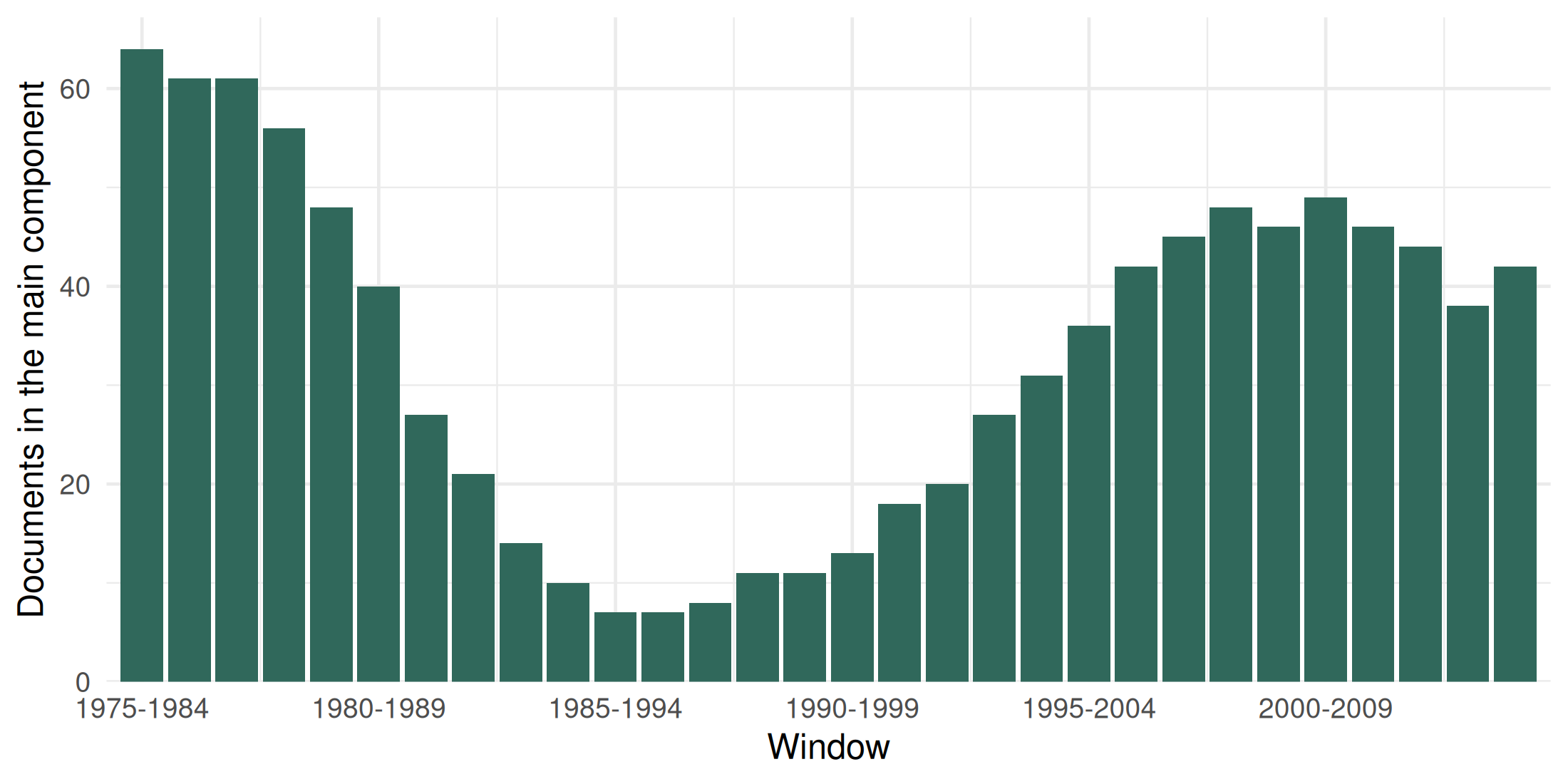
The size of the windows tells a story of its own: the stagflation was widely debated in the late 1970s and early 1980s, interest faded after the mid-1980s, and a new literature on it emerged in the 1990s, the pattern that Goutsmedt (2021) describes. It also warns about a technical limit: windows centred on the late 1980s contain about ten documents, too few for their clusters to mean much. The choice of the window is substantive. It should be long enough for each network to have enough documents to show a structure, and short enough for changes to be visible. Sliding windows smooth the evolution (consecutive networks share 90% of their period here) and make clusters easier to follow; successive windows give independent snapshots.