
library(networkflow)
library(ggplot2)
library(dplyr)
library(tidygraph)

nodes <- subset(Nodes_stagflation, source_type == "Stagflation")
network <- build_network(
  nodes = nodes,
  directed_edges = Ref_stagflation,
  source_id = "source_id",
  target_id = "target_id",
  method = "similarity",
  edges_threshold = 1
)This guide covers the second step of the pipeline: detecting clusters in a network and interpreting them. It starts from the bibliographic coupling network of the explanations of the 1970s stagflation built in the first guide.
What is a cluster?
In a bibliographic coupling network, a group of documents that cite the same literature, much more among themselves than with the rest of the network, is the usual operational definition of a research specialty or a research front (Morris and Van der Veer Martens 2008; Boyack and Klavans 2010). Detecting such groups without deciding them in advance is the task of community detection (Fortunato 2010). The algorithms differ, but most formalise “more ties inside than outside” with the modularity of a partition (Newman and Girvan 2004):
Q = \frac{1}{2m} \sum_{i,j} \left( A_{ij} - \gamma \frac{k_i k_j}{2m} \right) \delta(c_i, c_j),
with A_{ij} the weight of the edge between documents i and j, k_i the total weight of the edges of i, m the total weight of the network, \delta(c_i, c_j) = 1 when i and j are in the same cluster, and \gamma the resolution. The term k_i k_j / 2m is the weight expected between i and j if edges were placed at random given each node’s weight: a partition has a high modularity when clusters gather much more weight than expected by chance.
Detecting clusters with Leiden
add_clusters() gives access to five algorithms of igraph. The Leiden algorithm (Traag et al. 2019) is the default choice of recent bibliometric work. It improves on Louvain (Blondel et al. 2008) by guaranteeing that clusters are connected, and iterating it keeps refining the partition.
network <- add_clusters(
  network,
  clustering_method = "leiden",
  objective_function = "modularity",
  resolution = 1,
  seed = 123
)
Each document gets a cluster_leiden identifier and the share of the network that its cluster represents (size_cluster_leiden). Edges get the cluster of their two ends, or “00” when they connect two clusters.
node_table <- as_tibble(network, active = "nodes")
node_table |>
  count(cluster_leiden, name = "number_of_nodes", sort = TRUE) |>
  rename(community = cluster_leiden)
# A tibble: 4 × 2
community number_of_nodes
<chr> <int>
1 01 69
2 02 51
3 03 18
4 04 9The table gives, for each community (the cluster number, “01” being the largest), its number of nodes, that is of documents.
Resolution and the number of clusters
The partition depends on \gamma: a higher resolution makes the expected weight larger and favours more, smaller clusters. Modularity also has a resolution limit: in large networks, it can merge small communities that are clearly separated (Fortunato 2010). A network can legitimately be described at several levels of detail, from fields to specialties (Sjögårde and Ahlgren 2020), and choosing the resolution is choosing the level of the study. A scan of resolutions shows how the number of clusters reacts.
Leiden is also stochastic: two runs with different seeds can give different partitions. A partition we can trust should come back from one seed to the next. The adjusted Rand index (ARI) measures the agreement between two partitions, from about 0 (no more than chance) to 1 (identical). We run Leiden with ten seeds for each resolution and compare each partition with the one of the first seed.
scan <- expand.grid(resolution = seq(0.5, 2, by = 0.25), seed = 1:10)
memberships <- lapply(seq_len(nrow(scan)), function(i) {
  clustered <- add_clusters(
    network,
    clustering_method = "leiden",
    objective_function = "modularity",
    resolution = scan$resolution[i],
    seed = scan$seed[i],
    verbose = FALSE
  )
  as.integer(as_tibble(clustered, active = "nodes")$cluster_leiden)
})
scan$n_clusters <- sapply(memberships, function(m) length(unique(m)))
scan$ari <- sapply(seq_len(nrow(scan)), function(i) {
  reference <- which(scan$resolution == scan$resolution[i] & scan$seed == 1)
  igraph::compare(memberships[[i]], memberships[[reference]], method = "adjusted.rand")
})
scan_summary <- aggregate(cbind(n_clusters, ari) ~ resolution, data = scan[scan$seed != 1, ], FUN = mean)
scan_long <- rbind(
  data.frame(resolution = scan_summary$resolution, value = scan_summary$n_clusters, measure = "Mean number of clusters"),
  data.frame(resolution = scan_summary$resolution, value = scan_summary$ari, measure = "Mean ARI with seed 1")
)
ggplot(scan_long, aes(resolution, value)) +
  geom_line(colour = scico::scico(1, palette = "batlow", begin = 0.3), linewidth = 1) +
  geom_point(colour = scico::scico(1, palette = "batlow", begin = 0.3), size = 2.5) +
  facet_wrap(~measure, scales = "free_y") +
  scale_x_continuous(expand = expansion(mult = c(0.02, 0.02))) +
  labs(x = "Resolution", y = NULL) +
  theme_minimal(base_size = 16)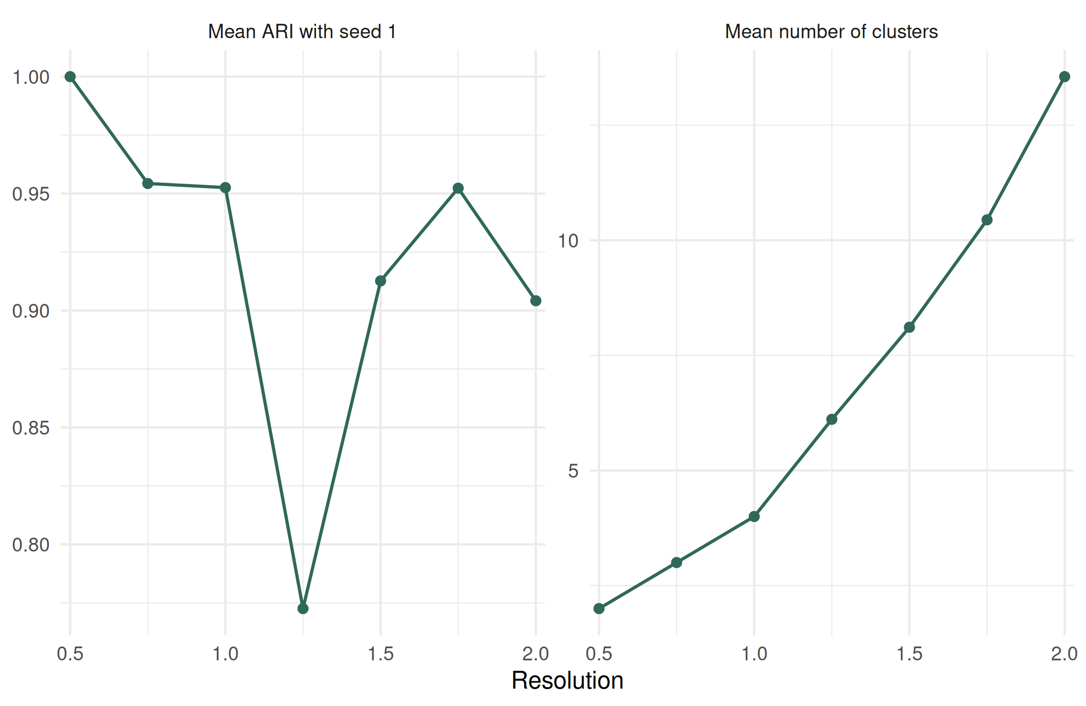
The number of clusters grows steadily with the resolution, and most resolutions give partitions that the seed hardly changes. Where the ARI drops, the algorithm hesitates between partitions of similar quality: results at that resolution should be read with care. A reasonable practice is to choose a resolution in a stable range, to report it, and to check that the clusters a narrative relies on survive at close values (Traag et al. 2013).
Modularity or CPM?
Leiden can also maximise the constant Potts model (Traag et al. 2011), which compares the internal weight e_c of each cluster with \gamma times its number of pairs: H = \sum_c [e_c - \gamma \binom{n_c}{2}]. A cluster is worth creating when its density exceeds \gamma. Unlike modularity, CPM does not depend on the size of the network, which helps when comparing clusters across networks of very different sizes, as time windows often are. But \gamma then lives on the scale of the edge weights:
edge_weights <- as_tibble(network, active = "edges")$weight
n_documents <- igraph::vcount(network)
density <- sum(edge_weights) / choose(n_documents, 2)
c(smallest = min(edge_weights), median = median(edge_weights), largest = max(edge_weights), density = density)
smallest median largest density
0.005403465 0.038992699 0.399613285 0.013310240 The weights of this network lie between 0.0054 and 0.4, so that a resolution of 1 asks clusters to be denser than any pair of documents can be: every document would be its own cluster. A natural scale for \gamma is the density of the network, here the mean weight over all the pairs of documents, \bar{w} = \sum_{ik} w_{ik} / \binom{n}{2} = 0.013. A cluster created with \gamma = \bar{w} is, on average, as dense as the whole network; with \gamma = 2\bar{w} or 3\bar{w}, it must be two or three times denser. The higher the multiple, the more the clusters split into small, very cohesive groups:
cpm_scan <- lapply(c(1, 2, 3), function(multiple) {
  clustered <- add_clusters(
    network,
    clustering_method = "leiden",
    objective_function = "CPM",
    resolution = multiple * density,
    seed = 123,
    verbose = FALSE
  )
  sizes <- as_tibble(clustered, active = "nodes") |>
    count(cluster_leiden, name = "number_of_nodes")
  tibble(
    resolution = multiple * density,
    multiple_of_density = multiple,
    clusters = nrow(sizes),
    largest_cluster = max(sizes$number_of_nodes),
    clusters_of_5_nodes_or_more = sum(sizes$number_of_nodes >= 5)
  )
})
bind_rows(cpm_scan)
# A tibble: 3 × 5
resolution multiple_of_density clusters largest_cluster clusters_of_5_nodes_…¹
<dbl> <dbl> <int> <int> <int>
1 0.0133 1 21 65 5
2 0.0266 2 28 50 9
3 0.0399 3 37 45 8
# ℹ abbreviated name: ¹clusters_of_5_nodes_or_moreAt the density of the network, CPM finds a few sizeable clusters, close to the readings of modularity, and a tail of small groups; at three times the density, the largest cluster is much smaller and most documents are in clusters that are too small to be read. The density gives a starting point, not a rule: as for modularity, the resolution has to be explored, and the clusters that a narrative relies on checked at neighbouring values.
Reading clusters
A cluster is a set of documents with shared references, not an interpretation. Reading it means going back to its documents: what they discuss, when, who wrote them, which references they share, and what distinguishes them from neighbouring clusters (Ding 2011).
Naming clusters with tf-idf
name_clusters() gives each cluster a provisional label. With method = "tf-idf", each cluster is treated as one document made of the titles of its members, and its label gathers the terms with the highest tf-idf (Spärck Jones 1972; Salton and Buckley 1988): terms frequent in the cluster and rare in the others,
\text{tf-idf}_{tc} = \frac{n_{tc}}{\sum_u n_{uc}} \times \log\frac{C}{\mathrm{df}_t},
with n_{tc} the count of term t in cluster c, C the number of clusters and \mathrm{df}_t the number of clusters where t appears.
network <- name_clusters(
  network,
  method = "tf-idf",
  cluster_id = "cluster_leiden",
  text_columns = "source_title",
  nb_terms_label = 3,
  clean_word_method = "lemmatize"
)
node_table <- as_tibble(network, active = "nodes")
clusters <- aggregate(
  as.integer(source_year) ~ cluster_leiden + cluster_label,
  data = node_table,
  FUN = function(year) c(documents = length(year), median_year = median(year))
)
clusters <- do.call(data.frame, clusters)
names(clusters)[3:4] <- c("documents", "median_year")
clusters[order(clusters$median_year), ]
cluster_leiden cluster_label documents median_year
3 01 productivity, unemployment, wage 69 1980
4 04 stagflation, inflation, change 9 1995
2 03 oil, great stagflation, price shock 18 2002
1 02 great inflation, stabilization, rule 51 2005The labels and the median years already sketch a history. Clusters of the late 1970s and early 1980s talk about productivity, oil, wages and unemployment; clusters centred on the 2000s about the “great inflation” and policy “rules”. This matches the account of Goutsmedt (2021): supply shocks and inflation inertia dominated the first explanations, and a new literature centred on the role of monetary policy emerged in the 1990s. Titles are short, and their words are not always informative (“great”, “comment”): labels are only a first guess. extract_tfidf() shows more terms per cluster, and abstracts, when available, give better labels than titles.
Other methods name a cluster after one of its documents. method = "tidygraph_functions" uses the most central document: the centrality is any function of tidygraph that computes a node measure, given as a call in tidygraph_function, and label_columns says which column of the node table makes the label. Here, each cluster is named after its document with the highest PageRank:
central <- name_clusters(
  network,
  method = "tidygraph_functions",
  tidygraph_function = tidygraph::centrality_pagerank(),
  cluster_id = "cluster_leiden",
  label_columns = c("source_author", "source_year")
)
as_tibble(central, active = "nodes") |>
  distinct(cluster_leiden, cluster_label) |>
  arrange(cluster_leiden)
# A tibble: 4 × 2
cluster_leiden cluster_label
<chr> <chr>
1 01 WACHTER-M_1978
2 02 VELDE-F_2004
3 03 BARSKY-R_2002
4 04 DELONG-B_1997 method = "given_column" does the same with the highest value of a column that you provide, such as the number of citations received within the corpus (order_by = "node_size", with compute_size = TRUE in build_network()).
The role of documents: hubs and bridges
Within a cluster, documents do not play the same role. Guimerà and Nunes Amaral (2005) propose to place each node with two measures. The within-module degree compares the weight \kappa_i of the ties of i with its own cluster s_i with that of the other members, z_i = (\kappa_i - \bar{\kappa}_{s_i}) / \sigma_{\kappa_{s_i}}. The participation coefficient P_i = 1 - \sum_s (k_{is} / k_i)^2, with k_{is} the weight of the ties of i with cluster s, is 0 when all ties stay in one cluster and approaches 1 when they spread evenly across clusters.
network <- add_node_roles(network, cluster_id = "cluster_leiden")
roles <- as_tibble(network, active = "nodes")
table(roles$roles)
 R1 ultra-peripheral        R2 peripheral R3 non-hub connector
                  12                  125                    9
   R5 provincial hub
                   1
ggplot(roles, aes(participation_coeff, within_module_z, colour = cluster_label)) +
  annotate("rect", xmin = -Inf, xmax = Inf, ymin = 2.5, ymax = Inf, alpha = 0.08) +
  geom_point(size = 2.5, alpha = 0.8) +
  scico::scale_colour_scico_d(palette = "batlow") +
  scale_x_continuous(expand = expansion(mult = c(0.01, 0.02))) +
  labs(x = "Participation coefficient", y = "Within-module degree (z-score)", colour = NULL) +
  theme_minimal(base_size = 16) +
  theme(legend.position = "bottom") +
  guides(colour = guide_legend(ncol = 2))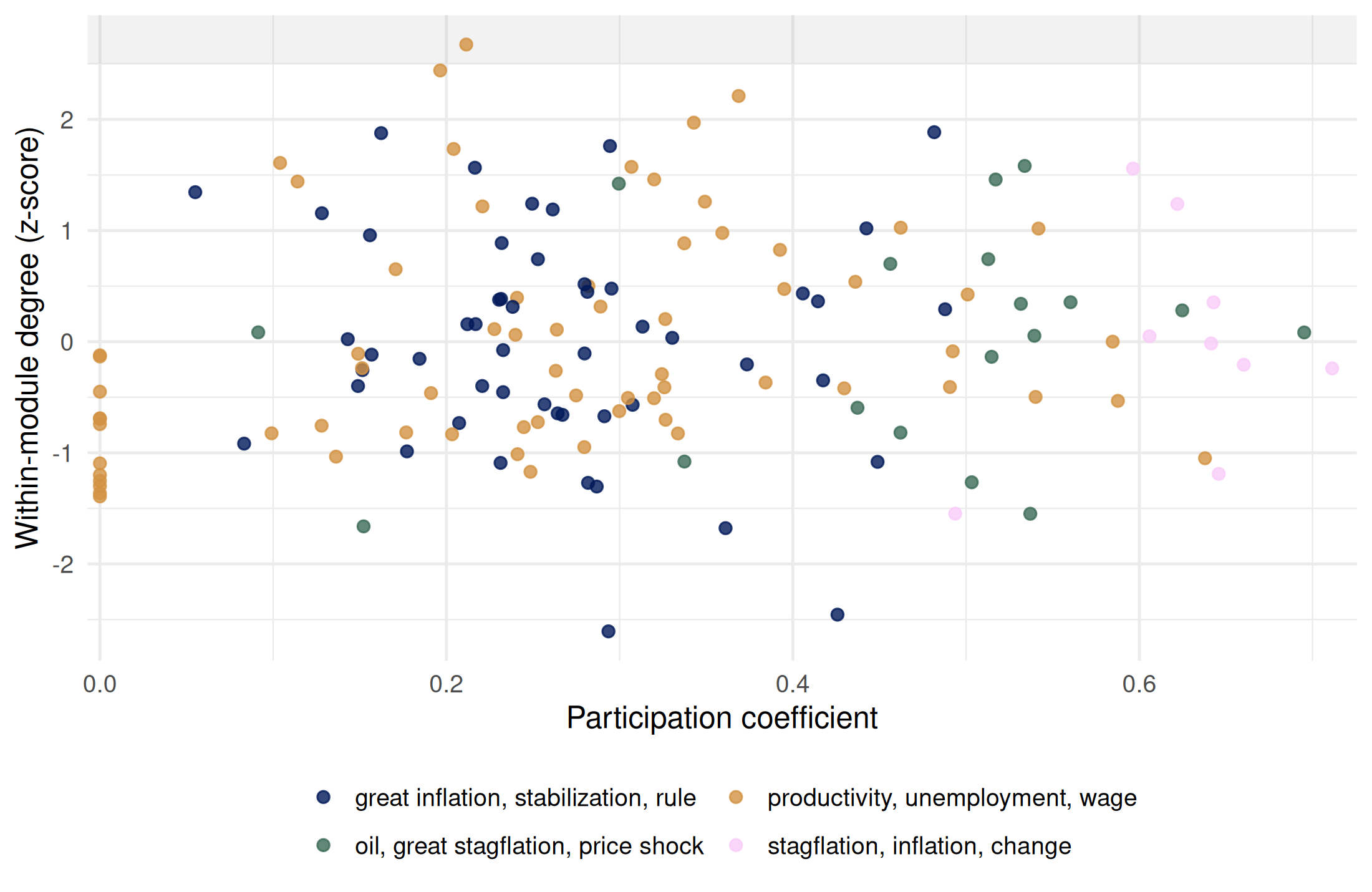
The shaded area holds the hubs of their cluster (z \geq 2.5, the threshold of Guimerà and Amaral). Documents on the right have ties spread over several clusters. The two measures combine into seven roles, which are easier to understand with documents in hand. Here are the documents that best illustrate the roles that exist in this network:
roles |>
  filter(roles %in% c("R5 provincial hub", "R6 connector hub", "R3 non-hub connector", "R4 non-hub kinless")) |>
  arrange(roles, desc(if_else(grepl("^R[567]", roles), within_module_z, participation_coeff))) |>
  group_by(roles) |>
  slice_head(n = 3) |>
  ungroup() |>
  transmute(role = roles, document = source_label, title = stringr::str_to_sentence(source_title),
            cluster = cluster_label, z = round(within_module_z, 1), participation = round(participation_coeff, 2)) |>
  as.data.frame()
role document
1 R3 non-hub connector BALL-L-1995a
2 R3 non-hub connector BLINDER-A-2013
3 R3 non-hub connector TAYLOR-J-1997
4 R5 provincial hub PINDYCK-R-1980
title
1 Relative-price changes as aggregate supply shocks
2 The supply-shock explanation of the great stagflation revisited
3 America<92>s peacetime inflation: the 1970s: comment
4 Energy price increases and macroeconomic policy
cluster z participation
1 stagflation, inflation, change -0.2 0.71
2 oil, great stagflation, price shock 0.1 0.70
3 stagflation, inflation, change -0.2 0.66
4 productivity, unemployment, wage 2.7 0.21How to read them depends on what the nodes and the ties are. Here, nodes are explanations of the stagflation and ties are shared references:
- A provincial hub (R5) is the central document of a literature: it shares references with most of the documents of its cluster and with hardly any other. Lansing’s “Exploring the causes of the great inflation”
- is one for the cluster on the great inflation, Nordhaus’s “Who’s afraid of a big bad oil shock?” (2007) for the cluster on oil. These are the documents to read first to enter a cluster.
- A connector hub (R6) is central in its cluster and shares references with others too. Pindyck’s “Energy price increases and macroeconomic policy” (1980) is central in the cluster on productivity, oil and supply while its references also belong to other clusters: a document built on several literatures that remains well embedded in one.
- A non-hub connector (R3) has ties spread over several clusters without being central in any: a bridge. Blinder’s “The supply-shock explanation of the great stagflation revisited” (2013) belongs to the cluster on oil but shares references with other clusters: it revisits an explanation that earlier documents had built on other bases. In a co-citation network, the same role belongs to works used by several literatures.
- A non-hub kinless document (R4) spreads its ties evenly over all clusters. This is not a better bridge than R3: it may be an outlier. The only one here, Nitzan’s article on “regimes of differential accumulation” (2001), shares references with each of five clusters in almost equal proportions (17 to 20% of its tie weight in each), and its within-module degree is below the average of its own cluster: it is tied to everybody a little and to nobody much.
Roles are positions in a network, not judgements on the importance of a document. Moreover, they depend on the partition. We recompute the roles for three resolutions of Leiden and follow the five documents above:
resolutions <- c(0.75, 1, 1.5)
by_resolution <- lapply(resolutions, function(resolution) {
  graph <- network |>
    add_clusters(clustering_method = "leiden", objective_function = "modularity",
                 resolution = resolution, seed = 123, verbose = FALSE) |>
    add_node_roles(cluster_id = "cluster_leiden")
  as_tibble(graph, active = "nodes") |> mutate(resolution = resolution)
})
bind_rows(by_resolution) |>
  group_by(resolution) |>
  summarise(
    clusters = n_distinct(cluster_leiden),
    hubs = sum(roles %in% c("R5 provincial hub", "R6 connector hub", "R7 kinless hub")),
    mean_participation = round(mean(participation_coeff), 2)
  ) |>
  as.data.frame()
resolution clusters hubs mean_participation
1 0.75 3 1 0.25
2 1.00 4 1 0.31
3 1.50 8 2 0.58
bind_rows(by_resolution) |>
  filter(source_label %in% c("LANSING-K-2000a", "NORDHAUS-W-2007", "PINDYCK-R-1980",
                             "BLINDER-A-2013", "NITZAN-J-2001")) |>
  select(document = source_label, resolution, roles) |>
  tidyr::pivot_wider(names_from = resolution, values_from = roles, names_prefix = "resolution ") |>
  as.data.frame()
document resolution 0.75 resolution 1
1 BLINDER-A-2013 R3 non-hub connector R3 non-hub connector
2 LANSING-K-2000a R2 peripheral R2 peripheral
3 NITZAN-J-2001 R3 non-hub connector R3 non-hub connector
4 NORDHAUS-W-2007 R2 peripheral R2 peripheral
5 PINDYCK-R-1980 R5 provincial hub R5 provincial hub
resolution 1.5
1 R4 non-hub kinless
2 R3 non-hub connector
3 R4 non-hub kinless
4 R2 peripheral
5 R6 connector hubWith smaller clusters, more ties cross clusters and the participation coefficients increase (the mean goes from 0.31 to 0.52). Blinder stays a connector at the three resolutions, and Lansing a hub, but Pindyck is only a peripheral document (R2) at 0.75 and a connector hub from 1. A role is therefore a statement about a document relative to a given partition: before interpreting a role in a text, check that it survives a reasonable change of resolution. Finally, the thresholds of Guimerà and Amaral were calibrated on metabolic networks. In a network of documents projected from references, a quarter of the pairs are tied, most documents have a participation above 0.05, and hubs are rare (three here): the roles are more useful as a way to find documents to read than as categories to count.
The same measures mean different things for other nodes: in a co-citation network, a hub is a classic cited with most of the works of its literature and a connector a work used by several literatures; for authors coupled through their references (see beyond bibliographic coupling), a connector is an author who cites several literatures.
What comes next
Clusters are easier to read on a map. The next guide shows how to compute the coordinates of the nodes, with several layouts, to colour the clusters and to draw the network. A single network of the whole period also mixes literatures that did not coexist: the last guide builds one network per time window and follows the clusters across windows.
References
Blondel, Vincent D., Jean-Loup Guillaume, Renaud Lambiotte, and Etienne Lefebvre. 2008. “Fast Unfolding of Communities in Large Networks.” Journal of Statistical Mechanics: Theory and Experiment 2008 (10): P10008. https://doi.org/10.1088/1742-5468/2008/10/P10008.
Boyack, Kevin W., and Richard Klavans. 2010. “Co-Citation Analysis, Bibliographic Coupling, and Direct Citation: Which Citation Approach Represents the Research Front Most Accurately?” Journal of the American Society for Information Science and Technology 61 (12): 2389–404. https://doi.org/10.1002/asi.21419.
Ding, Ying. 2011. “Community Detection: Topological Vs. Topical.” Journal of Informetrics 5 (4): 498–514. https://doi.org/10.1016/j.joi.2011.02.006.
Fortunato, Santo. 2010. “Community Detection in Graphs.” Physics Reports 486 (3): 75–174. https://doi.org/10.1016/j.physrep.2009.11.002.
Goutsmedt, Aurélien. 2021. “From the Stagflation to the Great Inflation: Explaining the US Economy of the 1970s.” Revue d’Économie Politique 131 (3): 557–82. https://www.cairn.info/revue-d-economie-politique-2021-3-page-557.htm.
Guimerà, Roger, and Luís A. Nunes Amaral. 2005. “Functional Cartography of Complex Metabolic Networks.” Nature 433 (7028): 895–900. https://doi.org/10.1038/nature03288.
Morris, Steven A., and Betsy Van der Veer Martens. 2008. “Mapping Research Specialties.” Annual Review of Information Science and Technology 42 (1): 213–95. https://doi.org/10.1002/aris.2008.1440420113.
Newman, M. E. J., and M. Girvan. 2004. “Finding and Evaluating Community Structure in Networks.” Physical Review E 69 (2): 026113. https://doi.org/10.1103/PhysRevE.69.026113.
Salton, Gerard, and Christopher Buckley. 1988. “Term-Weighting Approaches in Automatic Text Retrieval.” Information Processing & Management 24 (5): 513–23.
Sjögårde, Peter, and Per Ahlgren. 2020. “Granularity of Algorithmically Constructed Publication-Level Classifications of Research Publications: Identification of Specialties.” Quantitative Science Studies 1 (1): 207–38. https://doi.org/10.1162/qss_a_00004.
Spärck Jones, Karen. 1972. “A Statistical Interpretation of Term Specificity and Its Application in Retrieval.” Journal of Documentation 28 (1): 11–21.
Traag, V. A., G. Krings, and P. Van Dooren. 2013. “Significant Scales in Community Structure.” Scientific Reports 3: 2930. https://doi.org/10.1038/srep02930.
Traag, V. A., P. Van Dooren, and Y. Nesterov. 2011. “Narrow Scope for Resolution-Limit-Free Community Detection.” Physical Review E 84 (1): 016114. https://doi.org/10.1103/PhysRevE.84.016114.
Traag, V. A., L. Waltman, and N. J. van Eck. 2019. “From Louvain to Leiden: Guaranteeing Well-Connected Communities.” Scientific Reports 9 (1): 5233. https://doi.org/10.1038/s41598-019-41695-z.