The previous guides built one network and found its clusters. A single network of a long period, however, puts side by side literatures that never coexisted, and hides how a literature is born, grows, splits or fades. It can also build the wrong communities. In bibliographic coupling, two documents are tied by the references they share, and research tends to cite recent work: documents of the same years share more references than documents of different periods, whatever their topic. Over a long period, the communities then risk being communities of documents of the same period, rather than the thematic communities that one expects on a shorter window. Co-citation, where works are tied by the documents that cite them together, may suffer from a related problem, since these citing documents also belong to a period. This guide follows the dynamic workflow that is the core of networkflow: one network per time window, clusters in each window, and a rule that links the clusters of successive windows into dynamic clusters whose history can be told and drawn.
One network per window
We build bibliographic coupling networks of the explanations of the stagflation on sliding ten-year windows (1975-1984, 1976-1985…, 2004-2013), keep the main component of each, and detect clusters in each window with Leiden.
Each window has its own clusters, numbered “01”, “02”… These numbers mean nothing across windows: cluster “01” of 1975-1984 and cluster “01” of 1976-1985 may be two different literatures. Clusters are just ordered by their size in each window. Cluster “01” of 1975-1984 is the largest cluster of that window.
Linking clusters across windows
The rule
merge_dynamic_clusters() links each cluster to a cluster of the previous window when they share enough of their documents, and gives them a common identifier. Two rules are available, chosen with method, and the threshold and the type of similarity must be given explicitly. Let V_a be the documents of cluster a in window t-1, and V_b those of cluster b in window t.
The double majority (method = "majority"). Cluster b inherits the identifier of a when a majority of a goes to band a majority of b comes from a:
with \tau the threshold_similarity, strictly above 0.5 so that each cluster inherits at most one identifier and passes it to at most one cluster. The denominators depend on similarity_type:
"complete": D_a = |V_a| and D_b = |V_b|, all the documents of both clusters;
"partial": only the documents present in both windows count, D_a = |V_a \cap V_t| and D_b = |V_b \cap V_{t-1}|.
With overlapping windows, window t loses the documents of the first year of window t-1 and gains those of a new year. With "complete", a cluster that recruits many new documents, or loses many old ones, may lose its identifier because its composition changed. With "partial", only the documents present in both windows are compared, and a cluster that keeps its members together keeps its identifier however many documents join it. The first view treats a cluster as a group of documents, the second as a structure that recruits documents: which one fits depends on the question.
The Jaccard matching (method = "jaccard"), an overlap matching with a Jaccard threshold, as in the tracking of dynamic communities of Greene et al. (2010). The Jaccard index of two clusters is the share of their union that they have in common,
J(a, b) = \frac{|V_a \cap V_b|}{|V_a \cup V_b|},
and the pairs with J(a, b) \geq \theta are candidate matches. They are taken by decreasing J, skipping the pairs where a or b has already been matched, so that each past identifier goes to the present cluster that resembles it most and each cluster inherits at most one identifier. \theta can be well below 0.5: a cluster that loses a large part of its members to another cluster keeps its identity if it remains the best match of its predecessor. similarity_type = "partial" restricts the union to the documents present in both windows, as above.
The rules need documents present in successive windows. If windows follow each other without overlap (the default of build_dynamic_networks()), a network of documents shares no document from one window to the next (each document has a single year), and no cluster can be matched: the windows must overlap, that is window_step must be smaller than time_window (here window_step = 1).
window_networks<-networks# kept to compare other settings belownetworks<-merge_dynamic_clusters(window_networks, cluster_id ="cluster_leiden", node_id ="source_id", method ="majority", threshold_similarity =0.51, similarity_type ="partial")
How sensitive are the dynamic clusters to the threshold?
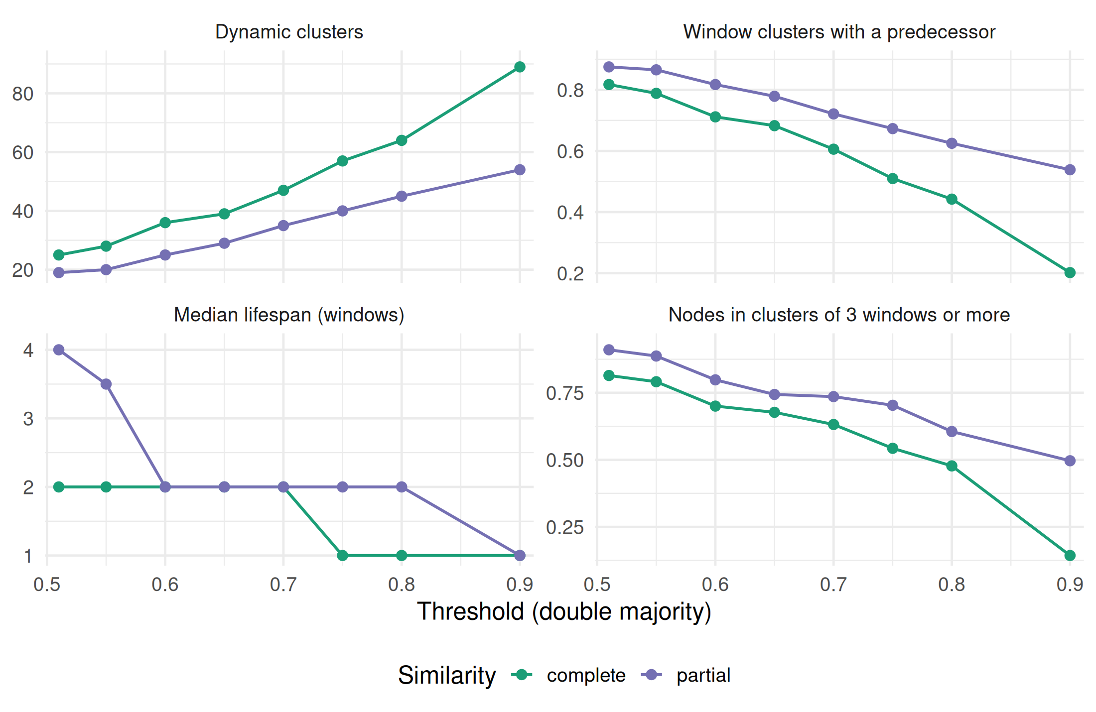
The threshold and the type of similarity decide how easily clusters are linked, hence how many dynamic clusters the history contains and how long they live. merge_diagnostics() runs the matching for a grid of thresholds and both similarity types, and plot_merge_diagnostics() draws the result.
The 110 window clusters become 25 dynamic clusters at 0.51 and 89 at 0.9 with the complete similarity (19 and 54 with the partial one): the more demanding the threshold, the more clusters are considered new. The curves are flat between 0.51 and 0.55, so that values just above 0.5 are on a plateau: the continuities they produce do not depend on the exact threshold. They bend after 0.55, and the second view below shows what is lost. With the complete similarity, the median lifespan falls to one window at 0.75: every window then has its own clusters, which is the opposite of a history. The partial similarity is more tolerant, because it ignores the documents that enter or leave the corpus from one window to the next. This is the reason for the thresholds just above 0.5 with partial similarity in the studies that used networkflow: 0.501 for Delcey et al. (2026), 0.55 for Duluins et al. (2026). Whatever the choice, the continuities that a narrative relies on should survive close thresholds, and a different seed of the clustering.
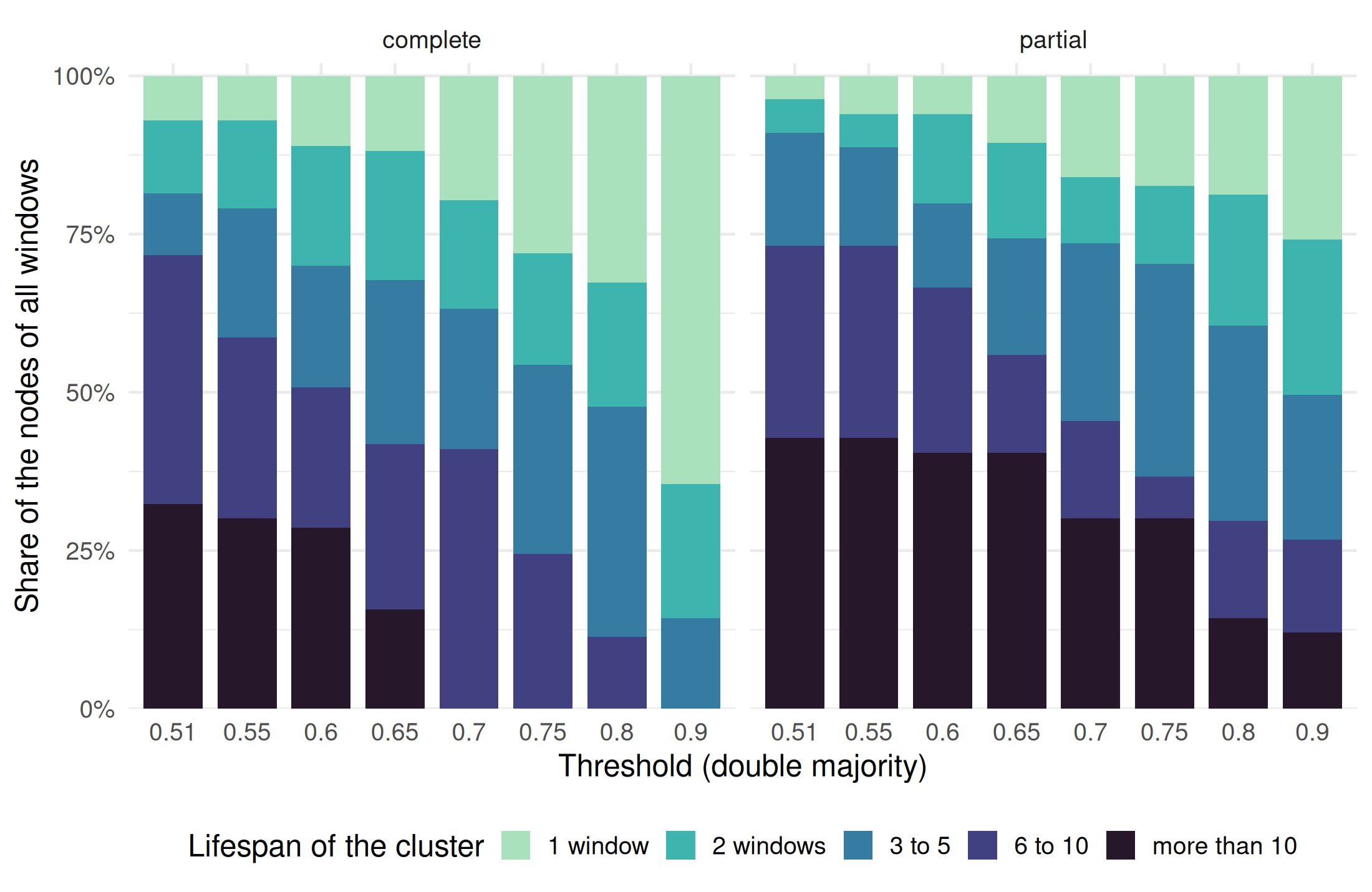
The second view shows who pays for a high threshold: the nodes of long clusters, which become members of short ones. With the complete similarity, the clusters that live more than ten windows gather about half of the nodes at 0.55 but 13% at 0.6, and none at 0.65: the longest continuities of the history are cut into shorter pieces between 0.55 and 0.65. With the partial similarity, such clusters still hold about 13% of the nodes at 0.9. The sensitivity of a continuity that matters for the story, here between 0.55 and 0.6, is exactly what the diagnostics are meant to reveal before it is hidden in a figure.
Comparing with the Jaccard matching
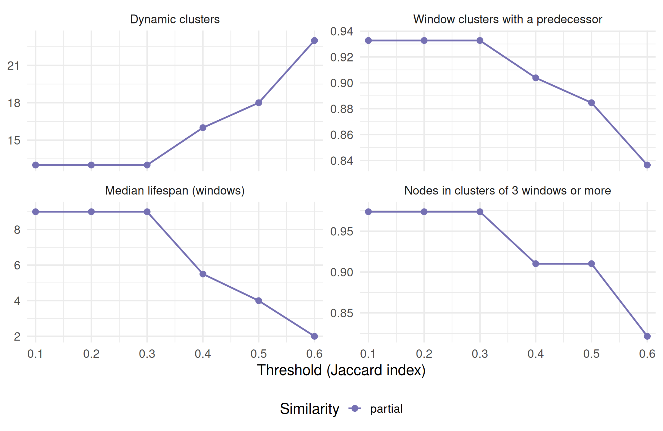
The same diagnostics exist for the Jaccard matching. Its threshold has a different meaning, so the grid is different (0.1 to 0.6): a Jaccard index of 0.3 means that clusters share 30% of their union, which is far below a majority.
To compare the two rules directly, we take the double majority at 0.51 and the Jaccard matching at a few thresholds, all with the partial similarity, and measure how much their dynamic clusters agree. The adjusted Rand index compares the dynamic cluster of each document in each window under two settings (1 for identical partitions, about 0 for no more agreement than chance).
The two rules largely agree on this corpus. The Jaccard matching is on a plateau from 0.1 to 0.3, where it finds 13 dynamic clusters, and breaks continuities beyond: 23 dynamic clusters at 0.6. At 0.5, it gives almost exactly the dynamic clusters of the double majority at 0.51 (an agreement of 1.00): a cluster that shares more than half of its union with its predecessor also shares a majority with it. The difference lies in the low thresholds. At 0.3, the Jaccard matching links clusters that the double majority leaves apart (13 dynamic clusters instead of 19, an agreement of 0.95), because a cluster whose members partly go elsewhere keeps its identity as long as it is the best match of its predecessor. Whether this is desirable depends on what a continuity is taken to be: a literature that loses part of its documents to another one, or two different literatures. Reading the documents of the clusters that only one rule links, rather than the indicators, is the way to decide.
Other ways to follow clusters
Both rules compare a cluster only with the previous window, so a cluster that vanishes for one window and comes back gets a new identifier. Splits and merges are not recorded as such: the part that meets the rule keeps the identifier, the others are new clusters. And the clusters of each window are detected independently, which adds instability between windows. Other approaches exist, which are not implemented in the package for now, but could be added and compared on the same data:
Detect communities in all windows at once, in a network where each node is tied to itself in adjacent windows with a coupling weight \omega. Identifiers are shared by construction.
The coupling \omega plays the role of the threshold, but clusters of one window are influenced by the neighbouring windows: more stable, less independent. It needs nodes present in several windows (co-citation, authors, journals rather than documents).
Bootstrap the network to find which clusters are robust, then draw the flows between robust clusters.
Addresses the instability of each partition rather than the matching rule; heavier.
Two simpler checks are available with the tools of the package: running the whole pipeline with several seeds of the clustering and comparing the dynamic clusters with merge_diagnostics(), and varying the window and its step (see the first guide), since instability often comes from windows that are too short to contain a stable structure.
Naming dynamic clusters
Once clusters are linked, each dynamic cluster can be named on all its documents across windows (name_dynamic_clusters = TRUE), with the words of the titles that distinguish it from the other dynamic clusters.
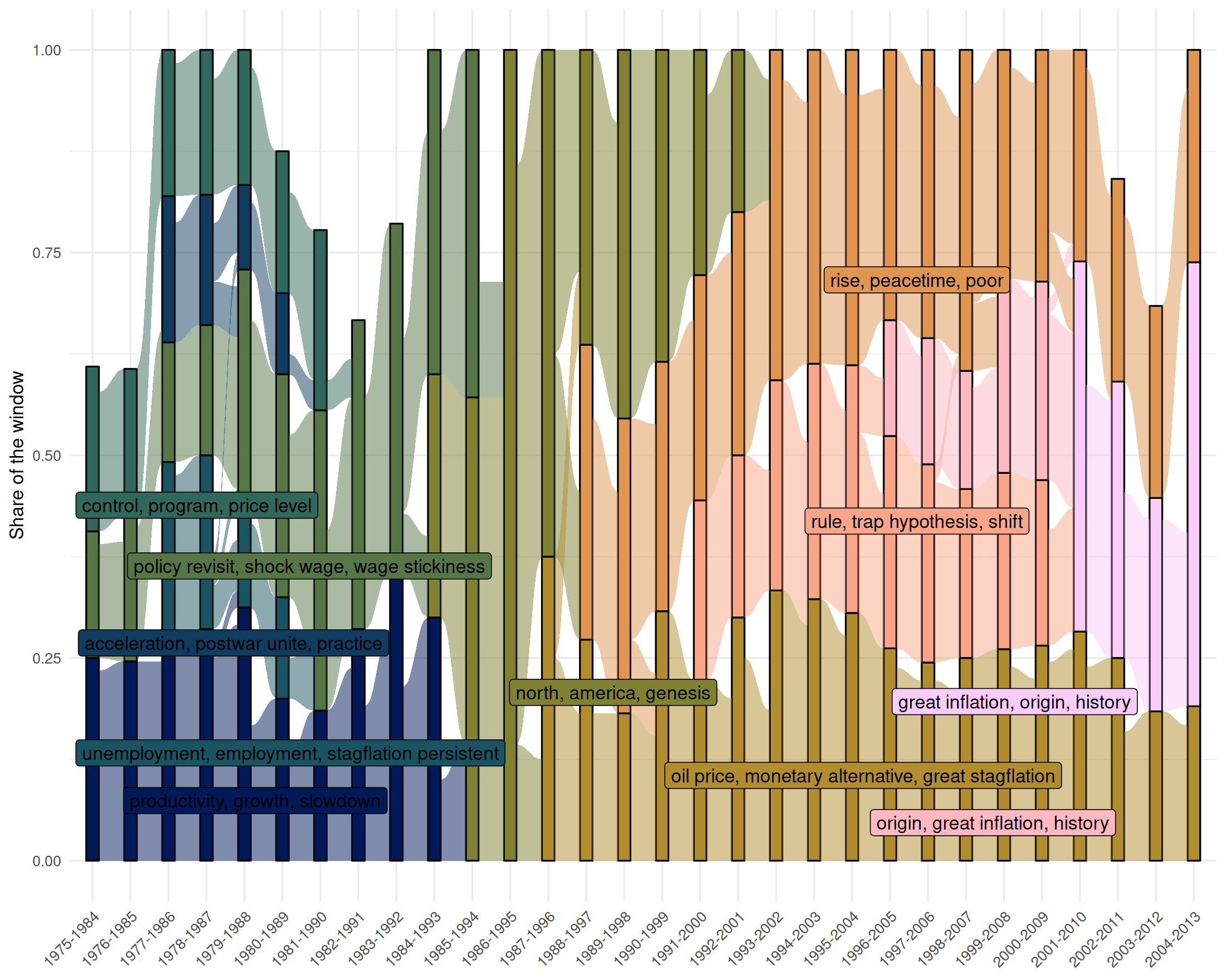
An alluvial plot shows the dynamic clusters as blocks in each window, with a height proportional to their share of the window, and flows that follow the documents from one window to the next. networks_to_alluv() stacks the node tables into the long table such a plot needs, with statistics on each cluster: its share of the whole history, its maximum share in a window, and the number of windows where it exists.
Clusters that exist in one or two windows, or remain small, clutter the plot. We keep the clusters that last at least three windows, give each a fixed colour, order the clusters to limit crossing flows (minimize_crossing = TRUE) and place each label in the middle of the cluster’s life (prepare_label = TRUE).
main_alluv<-alluv_dt[alluv_dt$length_cluster>=3, ]main_clusters<-sort(unique(main_alluv$dynamic_cluster_leiden))palette<-data.frame( dynamic_cluster_leiden =main_clusters, color =scico::scico(length(main_clusters), palette ="batlow"))plot_alluvial(main_alluv, cluster_id ="dynamic_cluster_leiden", node_id ="source_id", color_alluvial =TRUE, color =palette, minimize_crossing =TRUE, prepare_label =TRUE, cluster_label_column ="cluster_label")+labs(x =NULL, y ="Share of the window")+theme(axis.text.x =element_text(angle =45, hjust =1))
Figure 4
The plot draws the history that Goutsmedt (2021) tells with qualitative and quantitative methods. The early windows are shared between clusters on wages, productivity, controls and unemployment, the explanations of the late 1970s and early 1980s, centred on supply shocks and inflation inertia. These clusters fade in the late 1980s, when windows contain few documents. In the late 1980s and early 1990s, clusters on disinflation and on time-consistent policy bridge the two periods. From the 1990s, new clusters appear, on the “great inflation” and policy rules, on peacetime inflation, and on oil prices and monetary alternatives, and last until the end of the period: a new literature, centred on monetary policy, in which the contributions of new classical economists, ignored by the first explanations, became major references (Goutsmedt 2021).
Reading the plot requires care. Flows between clusters are documents that change cluster when the window slides, which may reflect a change in the literature or simply the instability of a partition of a small network. Windows of a dozen documents give fragile clusters: their part of the plot should be read with the documents in hand.
Coordinates that follow the documents
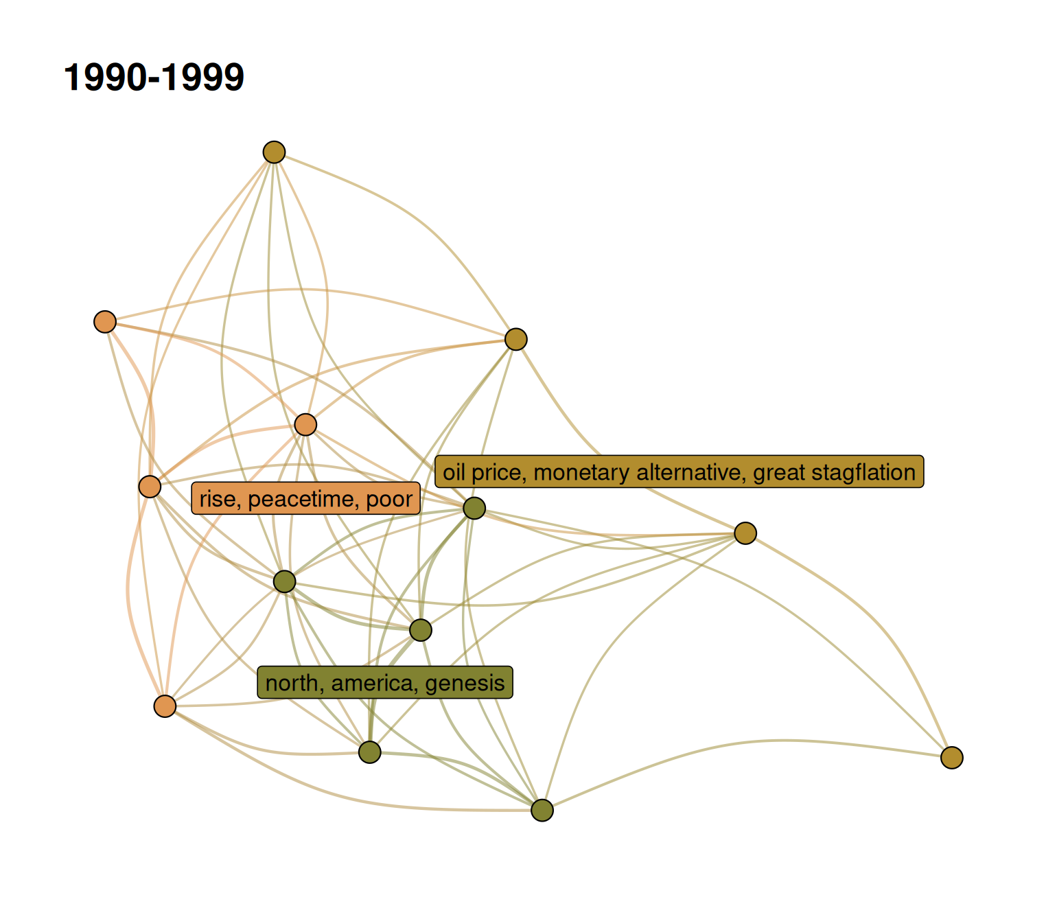
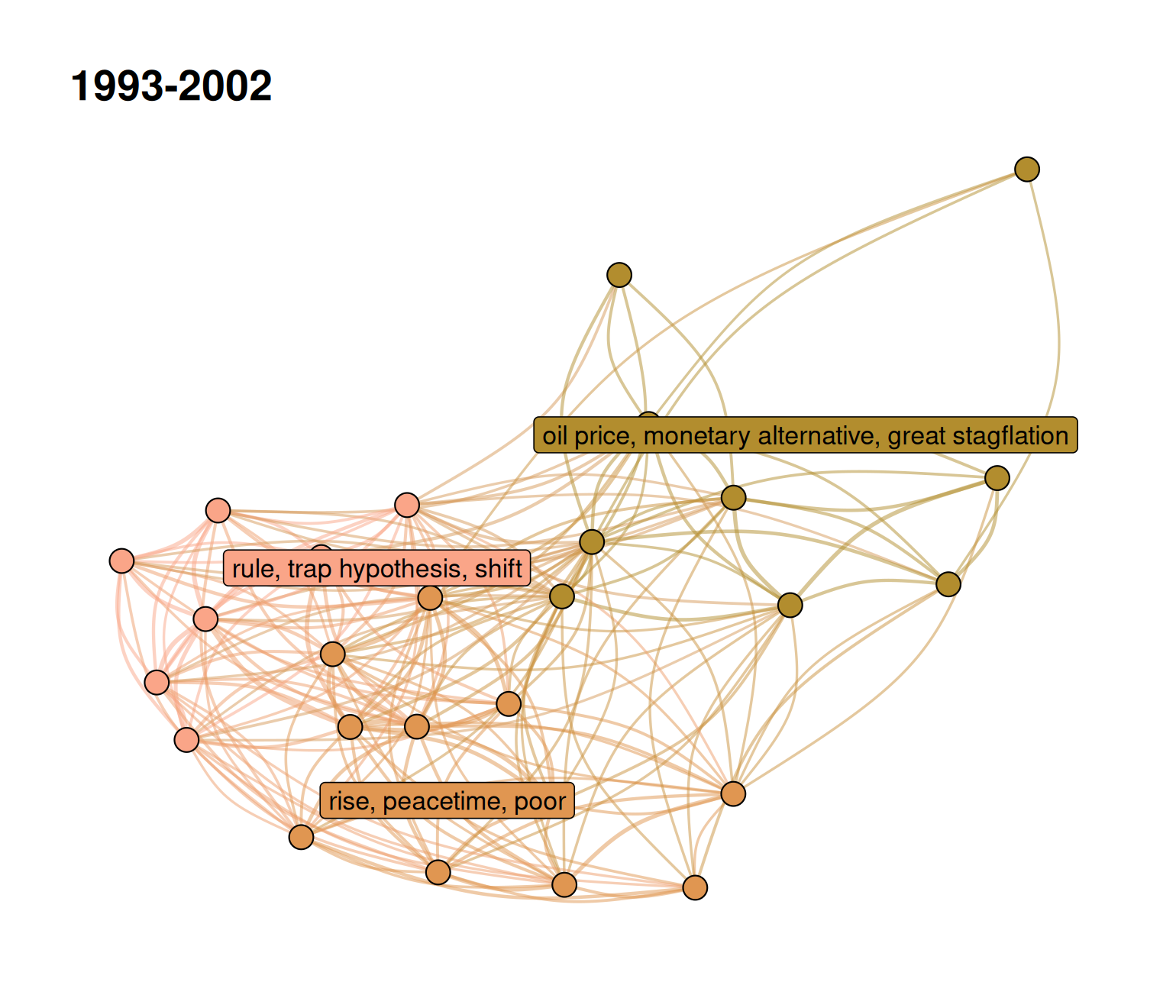
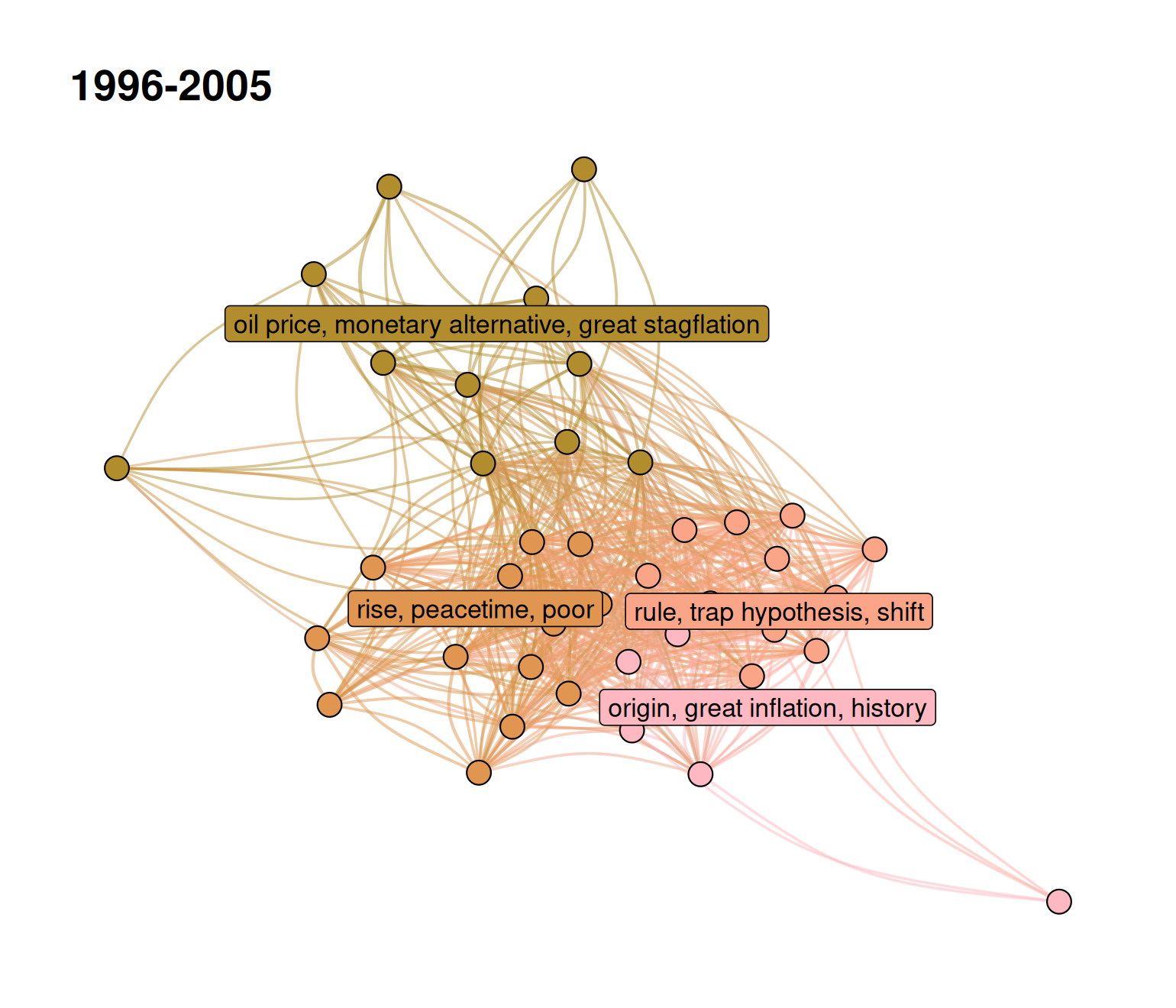
The alluvial shows the history of the clusters, but not the networks themselves. To look into the networks of successive windows side by side, the coordinates of a document should not jump from one plot to the next: an independent layout of each window would draw the same documents in unrelated places. layout_networks(compute_dynamic_coordinates = TRUE) starts the layout of each window from the coordinates of the previous one (documents new to the window start at the centre), so that a document tends to stay in the same region as long as it is in the corpus (see the guide on layouts). Giving the dynamic clusters the colours of the alluvial (color_networks() with the same palette, the small clusters being grey) completes the picture: a cluster can be followed in the alluvial and located in each network.
set.seed(1)networks<-layout_networks(networks, node_id ="source_id", layout ="fr", compute_dynamic_coordinates =TRUE)# the colours of the alluvial, and grey for the small clusters left out of itall_dynamic<-unique(unlist(lapply(networks, function(graph){as_tibble(graph, active ="nodes")$dynamic_cluster_leiden})))network_palette<-rbind(palette,data.frame( dynamic_cluster_leiden =setdiff(all_dynamic, palette$dynamic_cluster_leiden), color ="grey70"))networks<-color_networks(networks, column_to_color ="dynamic_cluster_leiden", color =network_palette, verbose =FALSE)shown<-c("1990-1999", "1993-2002", "1996-2005")plots<-plot_networks(networks[shown], cluster_label_column ="cluster_label", node_size_column =NULL)
Figure 5: Three windows, three years apart, with coordinates that follow the documents and the colours of the alluvial.
Successive windows share seven years out of ten, so most documents are present in the three plots and keep similar positions. The positions are not frozen, though: each layout starts from the previous one and moves the nodes again, so that a document can drift when its ties change. The layout must accept starting coordinates, which is the case of "fr", "kk" and "forceatlas2", not of "umap".
In research
The dynamic workflow was designed for histories of research fields, where the question is less “what are the communities?” than “when did a literature appear, what did it come from, and what did it become?”. Goutsmedt and Truc (2023) use bibliographic coupling and topic models to compare the macroeconomics published in the European Economic Review with the top five journals, between 1969 and 2002. Delcey et al. (2026) follow the discussions of rationality in a corpus of nearly 260,000 economics articles from 1900 to 2009. Duluins et al. (2026) apply the same tools to the scientific reception of a report on the environmental impact of livestock. In each case, the networks do not replace reading: they tell the historian which documents to read, and which continuities and breaks need an explanation.
References
Delcey, Thomas, Aurélien Goutsmedt, and Alexandre Truc. 2026. “One Sentence at a Time: A Quantitative History of Rationality in Economic Thought.”European Journal of the History of Economic Thought.
Duluins, Océane, Aurélien Goutsmedt, Noé Vandevoorde, and Philippe V. Baret. 2026. “A Scientometric Retrospective of the Livestock Long Shadow Report.”Frontiers in Sustainable Food Systems 9: 1656562. https://doi.org/10.3389/fsufs.2025.1656562.
Goutsmedt, Aurélien, and Alexandre Truc. 2023. “An Independent European Macroeconomics? A History of European Macroeconomics Through the Lens of the European Economic Review.”European Economic Review 158: 104559. https://doi.org/10.1016/j.euroecorev.2023.104559.
Greene, Derek, Dónal Doyle, and Pádraig Cunningham. 2010. “Tracking the Evolution of Communities in Dynamic Social Networks.”2010 International Conference on Advances in Social Networks Analysis and Mining, 176–83. https://doi.org/10.1109/ASONAM.2010.17.
Mucha, Peter J., Thomas Richardson, Kevin Macon, Mason A. Porter, and Jukka-Pekka Onnela. 2010. “Community Structure in Time-Dependent, Multiscale, and Multiplex Networks.”Science 328 (5980): 876–78. https://doi.org/10.1126/science.1184819.