
library(networkflow)
library(ggplot2)
library(dplyr)
library(tidygraph)

# The node table of a graph, whatever its active table
node_table <- function(graph) as_tibble(graph, active = "nodes")

nodes <- subset(Nodes_stagflation, source_type == "Stagflation")
refs <- Ref_stagflation
refs$source_id <- as.character(refs$source_id)
refs$target_id <- as.character(refs$target_id)

# One row per citation, with the year of the citing document
citations <- merge(refs[, c("source_id", "target_id")], nodes[, c("source_id", "source_year")], by = "source_id")
# One row per cited work
cited <- refs[!duplicated(refs$target_id), c("target_id", "target_author", "target_year", "target_title")]
cited$label <- paste0(cited$target_author, " (", cited$target_year, ")")The previous guides built bibliographic coupling networks: articles linked by the references they share. Nothing in the pipeline depends on this. The functions start from a table of links between two kinds of entities and project it onto one of them; clusters, dynamic matching, names, roles and plots then apply to whatever the nodes are. This guide shows three other uses on the same data: co-citation (cited works linked when they are cited together), author coupling (authors linked by the references of the documents they sign), and co-authorship, and explains the one data problem that matters more here than before: the identifiers of references.
Two sides of one table
A citation table links citing documents i to cited works j (a_{ij} = 1 when i cites j). Two projections are possible:
- on the citing documents, A A^\top: two documents are linked by the number of works they cite in common, |R_i \cap R_k|. This is bibliographic coupling (Kessler 1963);
- on the cited works, A^\top A: two works are linked by the number of documents that cite both, |C_j \cap C_l|, with C_j the set of documents citing j. This is co-citation (Small 1973).
Coupling is fixed when a document is published; co-citation changes as new documents cite old ones. Coupling maps the research fronts of a period, co-citation the intellectual base that the authors of a period build on. In build_network() and build_dynamic_networks(), the choice is made by projection_on: "source" (the default) links the source_id entities, "target" links the target_id entities.
Co-citation
The nodes are now the cited works, so the node table is the table of cited works. We keep the works that are cited together by at least four documents of the corpus, using the coupling angle (the cosine of the sets of citing documents), and ask compute_size to count the documents that cite each work.
cocitation <- build_network(
  nodes = cited,
  directed_edges = citations,
  source_id = "source_id",
  target_id = "target_id",
  projection_on = "target",
  method = "angle",
  edges_threshold = 4,
  compute_size = TRUE
)
cocitation <- filter_components(cocitation)
cocitation <- add_clusters(
  cocitation,
  clustering_method = "leiden",
  objective_function = "modularity",
  seed = 123,
  verbose = FALSE
)
c(works = igraph::vcount(cocitation), ties = igraph::ecount(cocitation))
works ties
108 572 Clusters of cited works are named after their most cited work (method = "given_column"), here the one with the most citing documents:
cocitation <- name_clusters(
  cocitation,
  method = "given_column",
  cluster_id = "cluster_leiden",
  label_columns = "label",
  order_by = "node_size"
)
node_table(cocitation) |>
  group_by(cluster = cluster_leiden, most_cited = cluster_label) |>
  summarise(works = n(), median_year = median(target_year, na.rm = TRUE), .groups = "drop") |>
  arrange(desc(works)) |>
  as.data.frame()
cluster most_cited works median_year
1 01 SARGENT-T (1998) 40 1999
2 02 CLARIDA, R, GALı´, J AND GERTLER, M. (2000) 25 2001
3 03 TAYLOR-J (1993) 21 1999
4 04 HAMILTON, J.D. (1983) 13 1995
5 05 FRIEDMAN, M. (1968) 7 1968
6 06 BARRO-R (1983) 2 1984Reading the most cited works of each cluster gives a map of the literature on which the explanations of the stagflation rely:
node_table(cocitation) |>
  group_by(cluster = cluster_leiden) |>
  slice_max(node_size, n = 2, with_ties = FALSE) |>
  transmute(cluster, work = label, title = target_title, cited_by = node_size) |>
  as.data.frame()
cluster work
1 01 SARGENT-T (1998)
2 01 DE LONG, BRADFORD (1997)
3 02 CLARIDA, R, GALı´, J AND GERTLER, M. (2000)
4 02 ORPHANIDES-A (1999)
5 03 TAYLOR-J (1993)
6 03 TAYLOR-J (1999)
7 04 HAMILTON, J.D. (1983)
8 04 BERNANKE, B. S., GERTLER, M., WATSON, M. (1997)
9 05 FRIEDMAN, M. (1968)
10 05 FRIEDMAN, M. (1977)
11 06 BARRO-R (1983)
12 06 BACKUS, D. AND DRIFFILL, J. (1985)
title
1 THE CONQUEST OF AMERICAN INFLATION
2 AMERICAS PEACETIME INFLATION: THE 1970S
3 MONETARY POLICY RULES AND MACROECONOMIC STABILITY: EVIDENCE AND SOME THEORY
4 THE QUEST FOR PROSPERITY WITHOUT INFLATION
5 DISCRETION VERSUS POLICY RULES IN PRACTICE
6 A HISTORICAL ANALYSIS OF MONETARY POLICY RULES
7 OIL AND THE MACROECONOMY SINCE WORLD WAR II
8 SYSTEMATIC MONETARY POLICY AND THE EFFECTS OF OIL PRICE SHOCKS
9 THE ROLE OF MONETARY POLICY
10 NOBEL LECTURE: INFLATION AND UNEMPLOYMENT
11 RULES DISCRETION AND REPUTATION IN A MODEL OF MONETARY POLICY
12 INFLATION AND REPUTATION
cited_by
1 32
2 32
3 28
4 26
5 22
6 18
7 13
8 12
9 20
10 8
11 8
12 4One cluster gathers the monetarist references of the 1960s and 1970s (Friedman’s 1968 presidential address, his Nobel lecture, his monetary history with Schwartz); one the works on oil shocks (Hamilton 1983, Bernanke, Gertler and Watson 1997); two the works on monetary policy rules, one around Taylor (1993, 1999) and one around Clarida, Galí and Gertler (2000) and Orphanides; one the works on the origins of the inflation of the 1970s and on the inconsistency of optimal policy (Sargent 1998, DeLong 1997, Kydland and Prescott 1977). A last, small cluster pairs two models of reputation (Barro 1983, Backus and Driffill 1985). This is the intellectual base of the explanations of the stagflation, seen through the works that their authors cite together, whereas the coupling network of the first guides mapped the explanations themselves.
set.seed(1)
cocitation <- layout_networks(cocitation, node_id = "target_id", layout = "fr")
clusters <- sort(unique(node_table(cocitation)$cluster_leiden))
cocitation <- color_networks(
  cocitation,
  column_to_color = "cluster_leiden",
  color = data.frame(cluster_leiden = clusters, color = scico::scico(length(clusters), palette = "batlow"))
)
plot_networks(cocitation, cluster_label_column = "cluster_label", node_size_column = "node_size")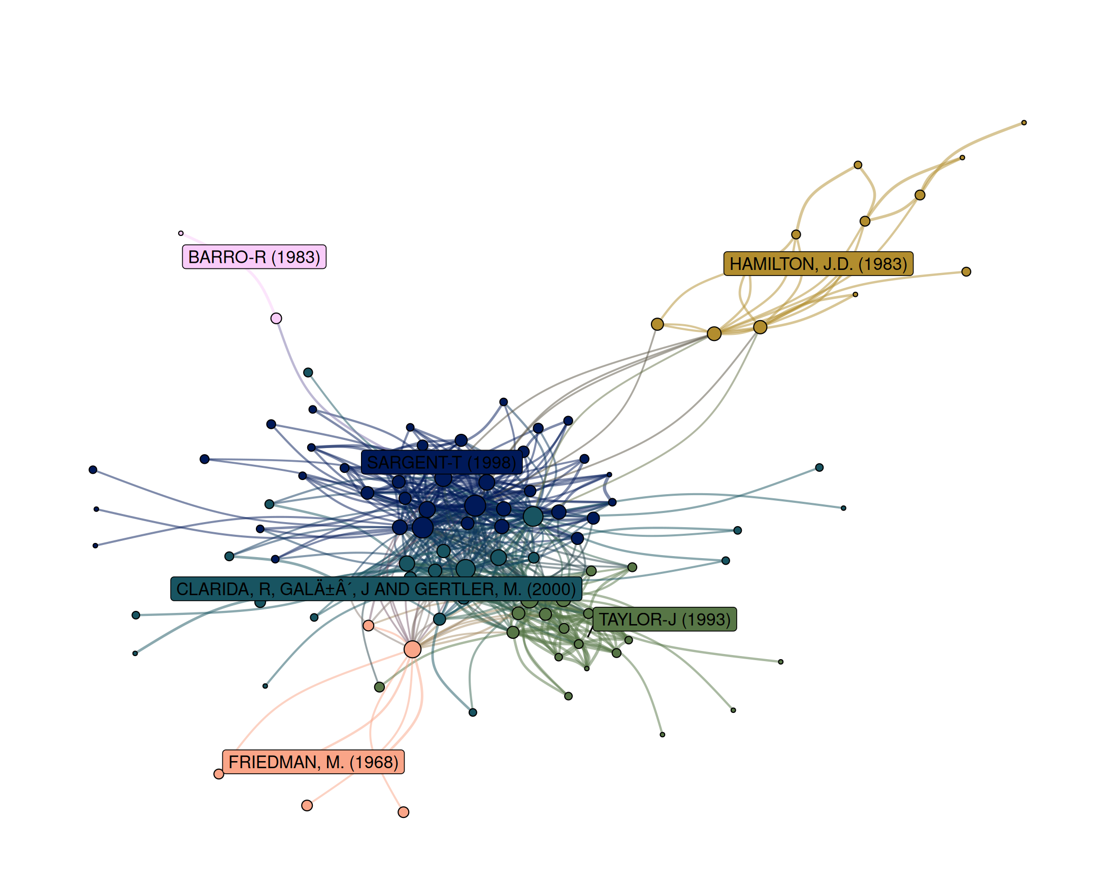
Identifiers of references
Every measure of the pipeline assumes that a work has one identifier: two documents are coupled by the references they share, and two works are co-cited by the documents that cite both. Raw bibliographic data break this assumption in two ways.
- One work, several spellings. The same article is written “FRIEDMAN, M. 1968. The role of monetary policy” in one bibliography, “Friedman, Milton. The Role of Monetary Policy.” in another. If the identifier of a reference is built from its text, each spelling is a different reference.
- Several works, one spelling. Truncated or incomplete references (“Friedman 1968”) may merge distinct works.
The consequences are not the same for the two projections. In coupling, a work split into several spellings loses some of the ties between the documents that cite it, but the nodes (the documents) are unaffected. In co-citation, the works themselves are the nodes: a work split into three spellings becomes three nodes, each cited by a fraction of its citing documents, each below the threshold, each without its true neighbours. The most cited works, which should be the hubs of the clusters, are the most likely to be written in many ways, and thus to be fragmented.
The problem is much smaller when the database gives an identifier to each cited reference, as Scopus, Web of Science or OpenAlex do when they match references to their records. In Ref_stagflation, Friedman’s article is written with six author strings, but it has a single target_id:
friedman <- refs[grepl("ROLE OF MONETARY POLICY", refs$target_title) & grepl("FRIEDMAN", refs$target_author), ]
c(citations = nrow(friedman),
  author_strings = length(unique(friedman$target_author)),
  identifiers = length(unique(friedman$target_id)))
citations author_strings identifiers
20 6 1 Identifiers are not perfect either: a database cannot match every reference, and may assign two identifiers to one work. A rough check compares the identifiers of works with the same title and year:
normalised <- paste(toupper(gsub("[^A-Za-z ]", "", refs$target_title)), refs$target_year)
usable <- !is.na(refs$target_title) & nchar(refs$target_title) > 12
ids_per_work <- tapply(refs$target_id[usable], normalised[usable], function(x) length(unique(x)))
c(works = length(ids_per_work), with_several_identifiers = sum(ids_per_work > 1))
works with_several_identifiers
1856 28 About 1.5% of the works have several identifiers. For the hubs of a co-citation network, it is worth looking at these cases by hand. In practice:
- use the identifiers of the database whenever there are any, and keep the reference text for labels only;
- without identifiers, build one from normalised fields (first author, year, source, volume, first page) rather than from the raw string, and merge identifiers that differ by a typo;
- look at the most cited works of the corpus, and of each cluster, for duplicates; they concentrate the damage;
- report the matching rule: the clusters depend on it.
Co-citation over time
A co-citation window should follow the citing documents: the network of 1988-2000 shows the works that the documents published in 1988-2000 cite together, whatever the date of the cited works. The year of the citing document is therefore a property of the links, not of the nodes: this is the role of time_in = "edges", where time_variable is a column of the table of links (here source_year, the year of the citing document). Cited works are nodes of any window where a link exists.
windows <- build_dynamic_networks(
  nodes = cited,
  directed_edges = citations,
  source_id = "source_id",
  target_id = "target_id",
  projection_on = "target",
  time_in = "edges",
  time_variable = "source_year",
  time_window = 13,
  method = "angle",
  edges_threshold = 3,
  compute_size = TRUE,
  filter_components = TRUE,
  verbose = FALSE
)
windows <- add_clusters(
  windows,
  clustering_method = "leiden",
  objective_function = "modularity",
  seed = 123,
  verbose = FALSE
)
vapply(windows, igraph::vcount, numeric(1))
1975-1987 1988-2000 2001-2013
12 16 158 The first two windows are tiny (12 and 16 works): the stagflation was a marginal topic between the mid-1980s and the mid-1990s, and few works are co-cited at least three times. Their clusters are fragile and the guide reads them as indications only.
The three windows are successive, not sliding, and this is possible because the nodes are cited works, which can appear in several windows: with coupling, successive windows share no document (each has a single date) and no cluster could be matched. Clusters of successive windows are linked through the cited works they share.
windows <- suppressWarnings(merge_dynamic_clusters(
  windows,
  cluster_id = "cluster_leiden",
  node_id = "target_id",
  method = "majority", threshold_similarity = 0.51,
  similarity_type = "partial"
))
windows <- name_clusters(
  windows,
  method = "given_column",
  name_dynamic_clusters = TRUE,
  cluster_id = "dynamic_cluster_leiden",
  label_columns = "label",
  order_by = "node_size"
)
bind_rows(lapply(windows, node_table), .id = "window") |>
  group_by(window, dynamic_cluster_leiden, most_cited = cluster_label) |>
  summarise(works = n(), .groups = "drop") |>
  arrange(window, desc(works)) |>
  group_by(window) |>
  slice_head(n = 4) |>
  as.data.frame()
window dynamic_cluster_leiden
1 1975-1987 cl_1
2 1975-1987 cl_2
3 1988-2000 cl_4
4 1988-2000 cl_3
5 1988-2000 cl_5
6 2001-2013 cl_5
7 2001-2013 cl_7
8 2001-2013 cl_3
9 2001-2013 cl_8
most_cited works
1 GORDON-R (1977) 7
2 GORDON-R (1973) 5
3 KYDLAND, F. E. AND E. C. PRESCOTT, (1977) 7
4 TAYLOR-J (1993) 6
5 SARGENT-T (1998) 3
6 SARGENT-T (1998) 52
7 ORPHANIDES-A (1999) 39
8 TAYLOR-J (1993) 34
9 CLARIDA, R, GALı´, J AND GERTLER, M. (2000) 28The two first windows share no cited work after the threshold: the works co-cited by the explanations of 1975-1987 (here, clusters named after Gordon’s 1973 and 1977 works) are not among those co-cited in 1988-2000, so no cluster of the first window is matched to a later one (merge_dynamic_clusters() warns about it, hidden here). The clusters of 1988-2000 around Taylor (1993) and Sargent (1998) are, on the other hand, found again in 2001-2013 under the same identifiers. This agrees with the history told by the coupling networks: a new literature, with its own references, replaces the first explanations. Co-citation shows that this literature relies on the works of a different intellectual base.
Authors instead of documents
Coupling can also be computed between entities that publish documents: authors, journals, institutions. The nodes are fewer and have a longer history than documents, and the question changes: who relies on the same literature, whatever the documents they write?
The table of links now has three columns: the entity (source_id, the author), the reference (target_id) and the document through which the author cites it (document_id). The last one matters because an author may cite a reference in several documents, and this counts more than one citation. Following Zhao and Strotmann (2008), entity_network() of biblionetwork (Goutsmedt et al. 2023) weights the tie between authors A and B by the number of times they cite the same references “together”. With C_{Aj} the number of documents of A citing reference j and L(A) = \sum_j C_{Aj} the total number of citations of A, the coupling angle is
w_{AB} = \frac{\sum_{j} \min(C_{Aj}, C_{Bj})}{\sqrt{L(A)\, L(B)}}.
authors <- Authors_stagflation
authors$source_id <- as.character(authors$source_id)

# One row per author, document and cited reference
by_author <- merge(authors, citations, by = "source_id")
author_nodes <- data.frame(author_name = unique(authors$author_name))
documents_per_author <- count(authors, author_name, name = "n_documents")

author_network <- build_network(
  nodes = author_nodes,
  directed_edges = by_author,
  source_id = "author_name",
  target_id = "target_id",
  document_id = "source_id",
  method = "strength",
  edges_threshold = 3
)
author_network <- filter_components(author_network) |>
  activate("nodes") |>
  left_join(documents_per_author, by = "author_name") |>
  add_clusters(clustering_method = "leiden", objective_function = "modularity", seed = 123, verbose = FALSE)

node_table(author_network) |>
  group_by(cluster = cluster_leiden) |>
  summarise(
    authors = n(),
    most_prolific = paste(head(author_name[order(-n_documents)], 4), collapse = ", ")
  ) |>
  as.data.frame()
cluster authors most_prolific
1 01 27 ORPHANIDES-A, MELTZER-A, TAYLOR-J, CUKIERMAN-A
2 02 22 BLINDER-A, NORDHAUS-W, KILIAN-L, BLANCHARD-O
3 03 17 SARGENT-T, COGLEY-T, WATSON-M, CECCHETTI-S
4 04 12 GORDON-R, MORK-K, FRYE-J, PERRY-G
5 05 8 CHRISTIANO-L, BALL-L, CHARI-V, MANKIW-G
6 06 8 RASCHE-R, TATOM-J, POOLE-W, DARBY-M
7 07 7 BRUNO-M, SACHS-J, MCCALLUM-C, HELLIWELL-J
8 08 6 IRELAND-P, DELONG-B, MAYER-T, VELDE-F
9 09 4 ROTEMBERG-J, GISSER-M, GOODWIN-T, WOODFORD-MThe groups are named after their most prolific authors. Orphanides and Taylor, whose works are among the most co-cited ones above, sit in the same group here, as authors who cite the same literature on monetary policy; Blinder, Nordhaus, Kilian and Blanchard form another group, and Gordon, Mork and Perry another. Whether such a group is a school, a generation or a topic is a question for the historian: the network only says who cites what.
Two cautions apply to entities. An article with several authors appears once for each of its authors, so co-authors are coupled by construction: a co-authorship network (below) tells how much of the coupling comes from joint work. And authors are heterogeneous aggregates: an author with one document has a short bibliography, an author with twenty has a long and diverse one. The coupling angle normalises by the total number of citations, but a threshold on the number of shared citations is easier to meet for prolific authors.
Because authors have no date, windows use the year of the documents they sign: time_in = "edges" with time_variable a column of the table of links, as for co-citation.
Co-authorship and other co-occurrences
The same function links entities by any two-mode relation. Authors linked by the documents they sign form a co-authorship network: the links are authors \to documents, and the shared “targets” are documents.
coauthorship <- build_network(
  nodes = author_nodes,
  directed_edges = authors,
  source_id = "author_name",
  target_id = "source_id",
  method = "angle"
)
c(authors = igraph::vcount(coauthorship), ties = igraph::ecount(coauthorship),
  components = igraph::components(coauthorship)$no)
authors ties components
78 64 29 documents_with_n_authors
1 2 3 5
123 38 9 1 Most explanations of the stagflation are single-authored (123 of the 171 documents with authors), so the co-authorship network is a set of small islands (29 components): it is not a useful network here, but a useful check, and in a corpus of articles in natural sciences or recent economics the picture would be very different. Other tables that fit this pattern include accounts and the hashtags they use, members and the boards they sit on, firms and the patents they hold, countries and the treaties they sign. In each case, choose which side becomes the nodes (projection_on), whether a measure of similarity or a statistical backbone is appropriate (see the first guide), and where time lies, in the nodes or in the links (time_in).
Summary
| You want to link… | Table of links | Main arguments |
|---|---|---|
| documents sharing references (coupling) | document \to reference | defaults |
| works cited together (co-citation) | document \to reference | projection_on = "target" |
| co-citation over the citing period | + year of the citing document | time_in = "edges" |
| authors sharing references | author, document, reference | document_id |
| authors signing the same documents | author \to document | defaults |
References
Goutsmedt, Aurélien, Alexandre Truc, and François Claveau. 2023. Biblionetwork: An R Package for Creating Different Types of Bibliometric Networks. Zenodo. https://doi.org/10.5281/zenodo.7677369.
Kessler, M. M. 1963. “Bibliographic Coupling Between Scientific Papers.” American Documentation 14 (1): 10–25. https://doi.org/10.1002/asi.5090140103.
Small, Henry. 1973. “Co-Citation in the Scientific Literature: A New Measure of the Relationship Between Two Documents.” Journal of the American Society for Information Science 24 (4): 265–69. https://doi.org/10.1002/asi.4630240406.
Zhao, Dangzhi, and Andreas Strotmann. 2008. “Author Bibliographic Coupling: Another Approach to Citation-Based Author Knowledge Network Analysis.” Proceedings of the American Society for Information Science and Technology 45: 1–10. https://asistdl.onlinelibrary.wiley.com/doi/full/10.1002/meet.2008.1450450292.