
library(networkflow)
library(ggplot2)
library(dplyr)

nodes <- subset(Nodes_stagflation, source_type == "Stagflation")
network <- build_network(
  nodes = nodes,
  directed_edges = Ref_stagflation,
  source_id = "source_id",
  target_id = "target_id",
  method = "similarity",
  edges_threshold = 2,
  filter_components = TRUE,
  verbose = FALSE
)
network <- add_clusters(
  network,
  clustering_method = "leiden",
  objective_function = "modularity",
  resolution = 1,
  seed = 123,
  verbose = FALSE
)
network <- name_clusters(
  network,
  method = "tf-idf",
  cluster_id = "cluster_leiden",
  text_columns = "source_title",
  nb_terms_label = 3,
  clean_word_method = "lemmatize"
)This guide covers the drawing of a network. A network has no natural position on a page: it is a set of nodes and of ties, and the figure we see depends on coordinates that something has to compute. This is the job of a layout, and the choice of the layout shapes what the reader sees. The guide starts from the bibliographic coupling network of the explanations of the 1970s stagflation built in the first guide, whose clusters were detected in the second one.
We keep the main component of a network with a threshold of two shared references (filter_components = TRUE): some layouts push the small, disconnected components far away from the rest, and the main component is the one we want to read.
What a layout does
A layout is a function that gives each node i a position p_i \in \mathbb{R}^2. Most layouts used in bibliometrics are force-directed: they treat the network as a physical system, in which tied nodes attract each other and all nodes repel each other, and look for positions where the forces balance. The clusters of a network, which are dense regions, then appear as groups of nodes close to each other. Venturini et al. (2019) insist that such a layout does not project the network on a space that exists beforehand: it creates the space, and they call the operation a “spatialisation”. Their guide to visual network analysis is the background of this one; Boullier et al. (2016) is a discussion in French that they cite on the visual structures a network can take.
layout_networks() computes the coordinates and adds them to the node table, in columns x and y. The layouts of igraph and graphlayouts are available through ggraph::create_layout(); "forceatlas2" and "umap" are added by networkflow.
Three cautions apply to all of them. First, layouts are stochastic (they start from random positions) and sensitive to their starting point: another seed gives another, equally valid picture, so set a seed before calling the function to reproduce a figure.
Second, distances in the picture are only roughly interpretable: nodes with more direct or indirect neighbours in common tend to be closer (Venturini et al. 2019). Two clusters drawn side by side are more tied than two clusters at opposite ends, but distances should not be measured. On their network of jazz musicians, Venturini et al. (2019) find that the distance between two nodes in a ForceAtlas2 layout is only loosely correlated with the length of the shortest path between them (R^2 = 0.17). Squeezing a network into two dimensions distorts it: four nodes all tied to each other cannot be drawn at equal distances on a plane. What should be read is not the position of a node, nor the distance between two nodes, but the density of nodes and its variations: dense regions (clusters), empty spaces between them (structural holes), and shapes that are not circular (polarisation).
Third, a force-directed layout has no axes. Unlike a correspondence analysis, it treats space as the same in every direction: there is no “top” or “left”, and a variable that varies from left to right in one cluster may vary from top to bottom in another (Venturini et al. 2019). With a few hundred nodes or more, a network is not read as a diagram, by following paths from node to node, but as a map of its structure: clusters, centres, margins and bridges. This is the reading that the layouts below are meant to serve.
Force-directed layouts
Fruchterman-Reingold
Fruchterman-Reingold ("fr") is the default choice of networkflow (Fruchterman and Reingold 1991). With d the distance between two nodes and k an ideal distance, every pair of nodes repels with a force k^2/d, and every pair of tied nodes attracts with a force d^2/k, multiplied by the weight of the tie in igraph: heavier edges pull nodes closer.
set.seed(1)
laid_out <- layout_networks(network, node_id = "source_id", layout = "fr")
head(as_tibble(laid_out, active = "nodes")[c("source_id", "cluster_leiden", "x", "y")])
# A tibble: 6 × 4
source_id cluster_leiden x y
<chr> <chr> <dbl> <dbl>
1 96284971 04 -5.02 -3.05
2 214927 05 -8.54 3.65
3 2207578 05 -2.93 5.91
4 10729971 05 -6.48 1.68
5 95575910 03 -0.0142 1.73
6 105203318 03 1.66 1.71Kamada-Kawai, and a trap with weights
Kamada-Kawai ("kk") takes the opposite approach (Kamada and Kawai 1989): it places the nodes so that their geometric distances reproduce their graph distances, as if each pair of nodes were joined by a spring whose rest length is the length of the shortest path between them. The trap is that igraph reads the weight column of the edges as a distance for this layout, whereas a similarity is the opposite of a distance: the most similar documents would be pushed apart, and the weakly tied ones drawn at the margins. With similarity weights, either use "fr" or ignore the weights with weights = NA.
ForceAtlas2
ForceAtlas2 ("forceatlas2") is the layout of the visualisation software Gephi, designed for the exploration of networks (Jacomy et al. 2014). Its forces are close to those of Fruchterman-Reingold, with two differences that matter for bibliographic networks. The repulsion between two nodes grows with the product of their degrees: with \deg_i the number of ties of node i and d_{ij} the distance between i and j,
F_{\text{repulsion}}(i, j) = k_r \, \frac{(\deg_i + 1)(\deg_j + 1)}{d_{ij}}, \qquad F_{\text{attraction}}(i, j) = w_{ij} \, d_{ij},
so that hubs, which have many ties, push other nodes away more strongly than peripheral nodes do. A gravity F_{\text{gravity}}(i) = k_g (\deg_i + 1) keeps the nodes around the centre. Finally, the speed of the nodes adapts to the stability of the system: it increases when forces are consistent and decreases when nodes oscillate.
set.seed(1)
laid_out_fa2 <- layout_networks(network, node_id = "source_id", layout = "forceatlas2")
The implementation of networkflow is compact: it computes the repulsion between all the pairs of nodes, instead of the approximation of Gephi, so that its cost grows with the square of the number of nodes: on a sample of the Web of Science, about a minute for 1,000 nodes and four to five minutes for 2,000, when Fruchterman-Reingold and UMAP take a few seconds. For larger networks, prefer them. Three arguments change the picture: scaling_ratio is the strength of the repulsion k_r (smaller values give a more compact layout), linlog = TRUE replaces the attraction by a logarithm of the distance, which separates clusters more, and strong_gravity = TRUE keeps disconnected components close to the centre.
Venturini et al. (2019) show, on their jazz network, how much these settings matter: a network that looks like a “hairball” with Fruchterman-Reingold acquires a clearer structure with ForceAtlas2, especially with the LinLog mode and a lower gravity. Gravity prevents disconnected nodes from drifting away, but too much of it packs all the nodes in the centre; the LinLog mode with no gravity makes clusters more visible, but scatters the network and takes longer to converge. There is no setting that suits all networks: what first looks like a homogeneous tangle may come from an unfortunate choice of algorithm or settings, and the settings are to be adjusted to the network at hand.
UMAP
UMAP (Uniform Manifold Approximation and Projection) is not a graph layout: it is a method to embed points in a low-dimensional space while preserving their neighbourhoods (McInnes et al. 2018). The two families are not as far apart as they seem: Venturini et al. (2019) note that dimensionality reduction methods such as t-SNE and UMAP implicitly build a network of neighbours and spatialise it, by an iterative relaxation that resembles force-directed layouts. It often gives nice visualisations, with compact and well separated clusters. It needs distances between points, which a network does not provide directly, so layout_networks() builds them from the network: the distance between two nodes is the length of the shortest path between them, an edge being as long as the inverse of its weight (a strong tie is a short one). UMAP then describes each node by its n_neighbors nearest nodes and finds coordinates that reproduce this neighbourhood structure.
set.seed(1)
laid_out_umap <- layout_networks(network, node_id = "source_id", layout = "umap", n_neighbors = 15)
n_neighbors is the size of the neighbourhood that is preserved: small values emphasise local structure and many small groups, large values a global view of the network. min_dist (0.1 by default) sets how tightly nodes are packed. The picture is thus partly built by the user, and a UMAP should be checked with several values of n_neighbors. Unlike force-directed layouts, UMAP does not put the nodes of two components close by default: nodes of different components are set farther apart than any connected pair. The package uwot computes it, and must be installed.
Comparing the layouts
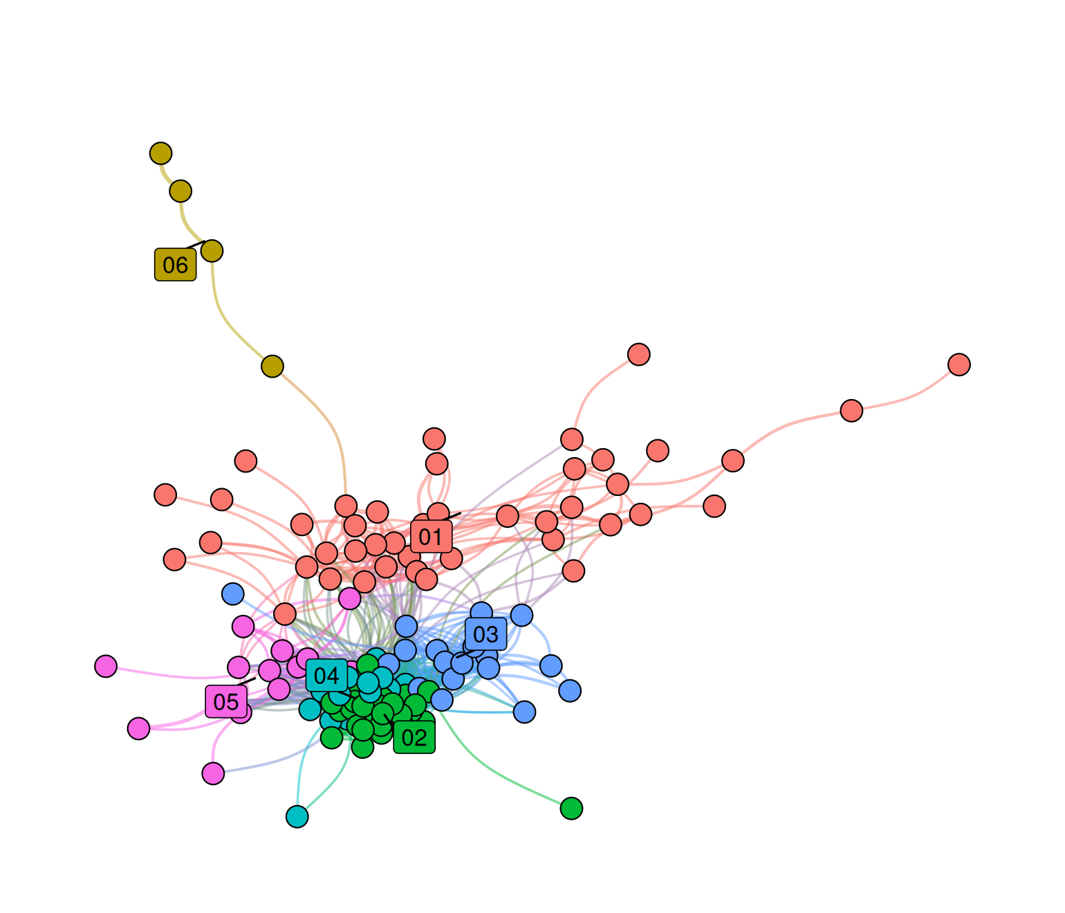
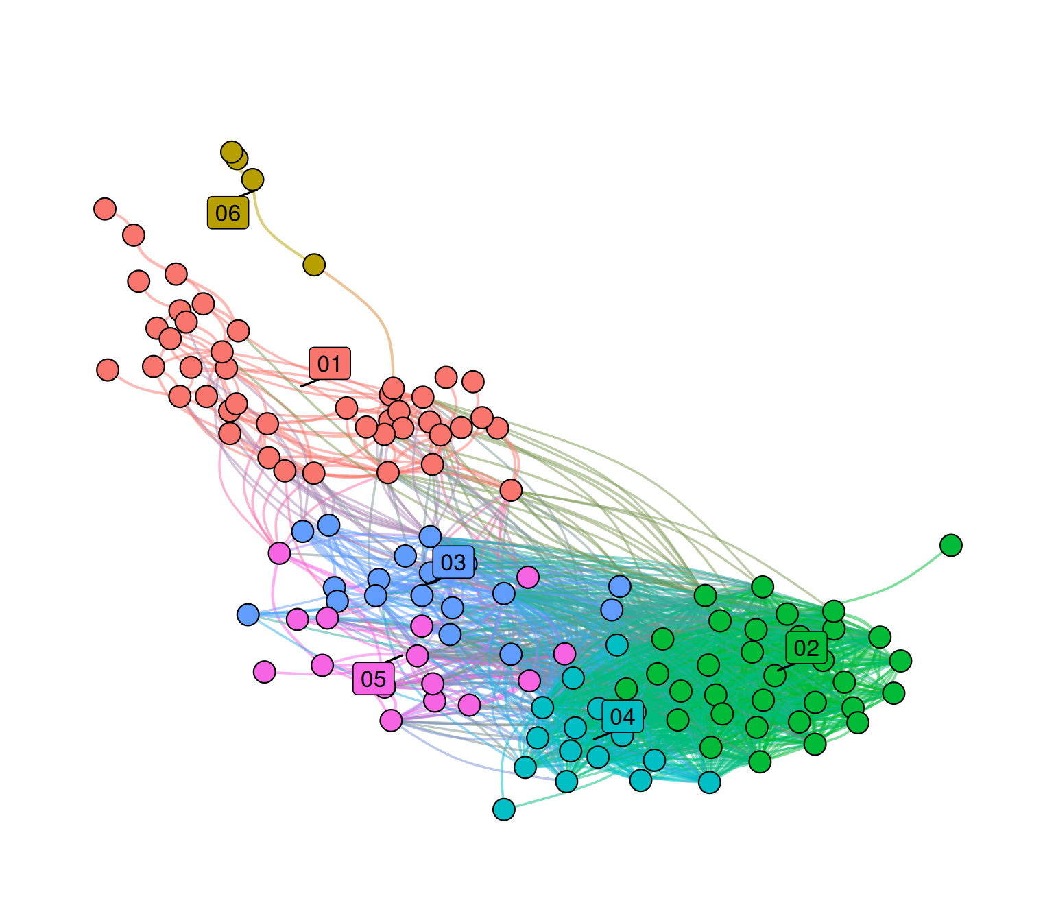
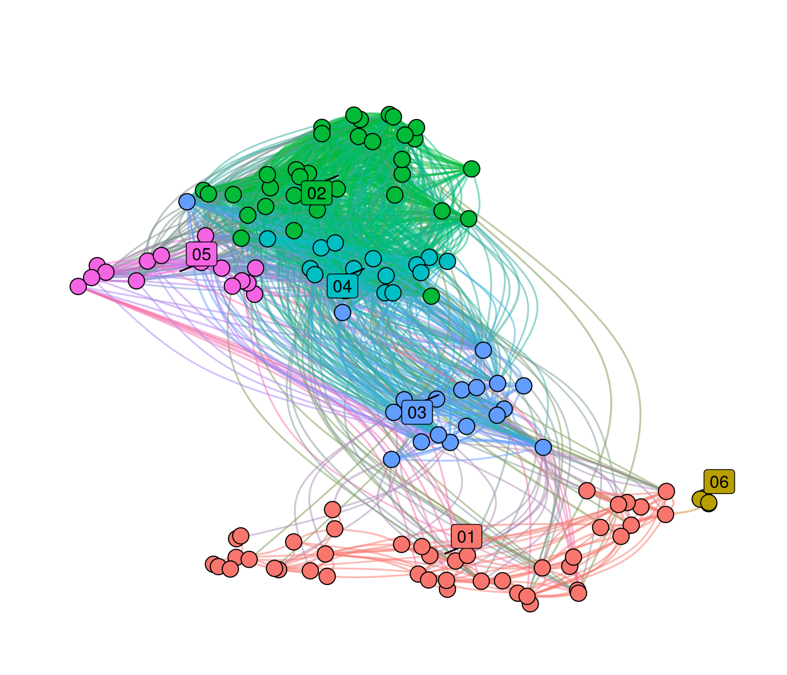
The same network, with the same clusters, in three layouts, each node being coloured by its Leiden cluster (the labels are the cluster numbers).
network <- color_networks(network, column_to_color = "cluster_leiden", verbose = FALSE)
for (layout in c("fr", "forceatlas2", "umap")) {
  set.seed(1)
  laid_out <- layout_networks(network, node_id = "source_id", layout = layout)
  print(plot_networks(laid_out, cluster_label_column = "cluster_leiden", node_size_column = NULL))
}
None of them is the right one: they answer different questions.
| Layout | Idea | Uses the weights | Cost | Reads well when |
|---|---|---|---|---|
"fr" |
attraction along edges, repulsion between all nodes | as attraction | light | a first look at a network of a few hundred nodes |
"kk" |
geometric distances reproduce graph distances | as distances (see above) | grows fast with size | small networks, unweighted or with weights = NA
|
"forceatlas2" |
as "fr", with a repulsion that grows with degrees |
as attraction | square of the number of nodes: networks up to about 1,000 nodes | networks with hubs, which need space |
"umap" |
preserves the neighbourhood of each node | through the shortest paths | light | networks of clusters one wants to see apart |
How to tell whether a layout is good? There is no accepted measure of the quality of a spatialisation (Venturini et al. 2019). They suggest a simple heuristic: a good layout should give a visual partition of the network that roughly corresponds to its structural clustering. They cut the picture into groups with the k-means algorithm, with as many groups as Louvain finds clusters, and compare the two partitions. We do the same with the Leiden clusters, measuring the agreement with the adjusted Rand index (1 for identical partitions, about 0 for no more than chance; Venturini et al. (2019) use a Jaccard index of the pairs of nodes, in the same spirit).
cluster_ids <- as.integer(factor(as_tibble(network, active = "nodes")$cluster_leiden))
layout_check <- do.call(rbind, lapply(c("fr", "kk", "forceatlas2", "umap"), function(layout) {
  set.seed(1)
  laid_out <- if (layout == "kk") {
    layout_networks(network, node_id = "source_id", layout = layout, weights = NA)
  } else {
    layout_networks(network, node_id = "source_id", layout = layout)
  }
  coordinates <- as_tibble(laid_out, active = "nodes")[c("x", "y")]
  set.seed(1)
  groups <- kmeans(coordinates, centers = max(cluster_ids), nstart = 20)$cluster
  data.frame(
    layout = layout,
    agreement_with_leiden = igraph::compare(groups, cluster_ids, method = "adjusted.rand")
  )
}))
layout_check[order(-layout_check$agreement_with_leiden), ]
layout agreement_with_leiden
3 forceatlas2 0.5645819
4 umap 0.5502986
1 fr 0.3762415
2 kk 0.3311174On this network, forceatlas2 gives the picture whose regions best match the Leiden clusters. The heuristic has limits that Venturini et al. (2019) point out: it works on clearly clustered networks, less on networks with polarisations but no clear-cut clusters, and a layout is also valuable for what a partition cannot show, the gradients and the uncertain borders between groups. A practical rule: try a force-directed layout first, and a UMAP to check whether the clusters found by Leiden also appear as separate groups of nodes. When a cluster is split or scattered in all the layouts, it is worth reading its documents again.
Colours and labels
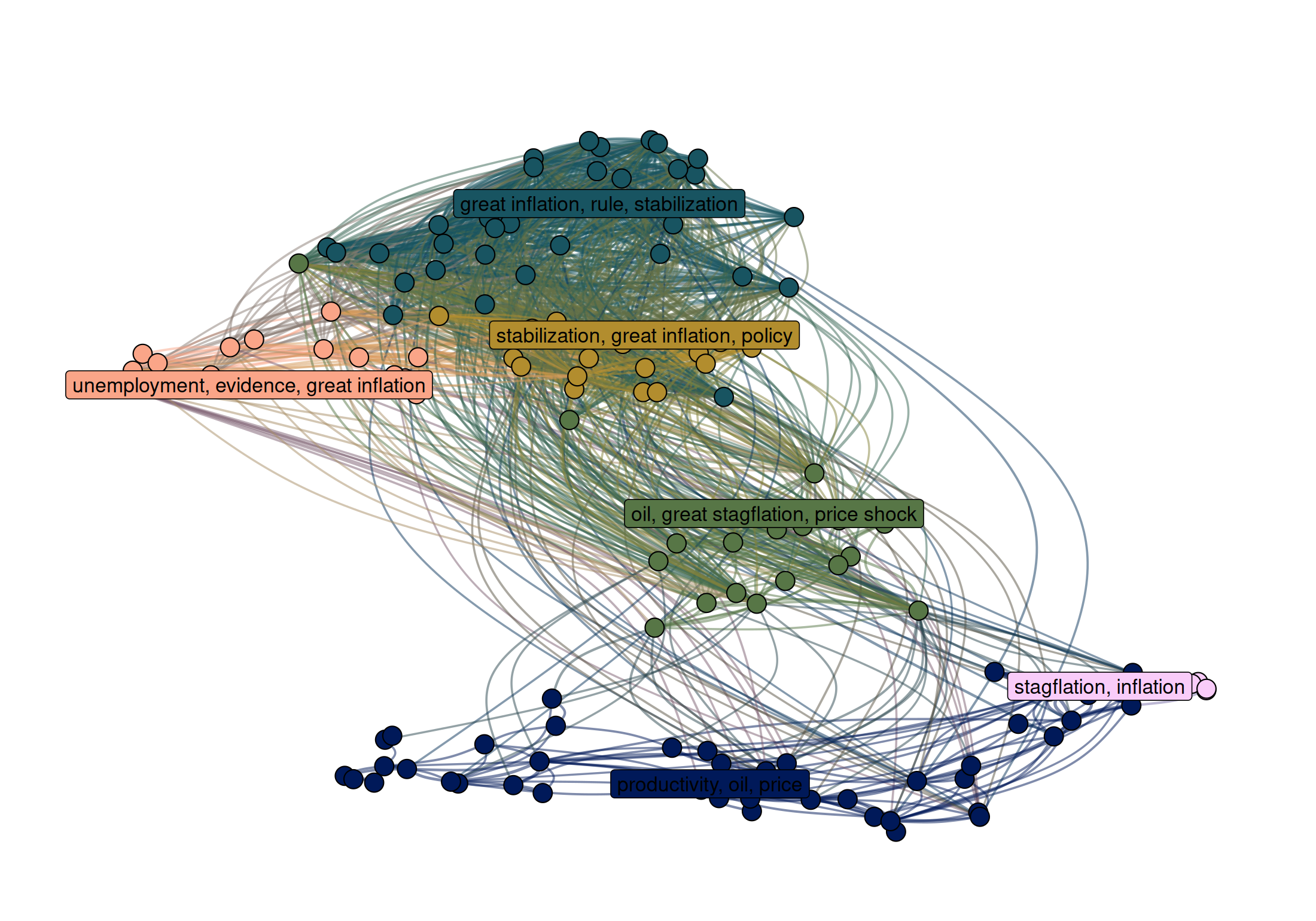
Position is the first visual variable of a network map; Venturini et al. (2019) describe two others, size and colour, which by convention follow the importance of a node and its category. Here, the category is the cluster. color_networks() gives each cluster a colour, in the order of decreasing size of the clusters, and each edge a mix of the colours of its two ends. The colours are the ones of a palette that you can choose, here the perceptually uniform batlow palette of scico, and a category keeps its colour in every figure if the palette is given explicitly.
n_clusters <- length(unique(as_tibble(network, active = "nodes")$cluster_leiden))
palette <- data.frame(
  cluster_leiden = sort(unique(as_tibble(network, active = "nodes")$cluster_leiden)),
  color = scico::scico(n_clusters, palette = "batlow")
)
network <- color_networks(network, column_to_color = "cluster_leiden", color = palette, verbose = FALSE)
The label of each cluster is drawn at the centre of gravity of its nodes: prepare_label_networks() computes these positions, and plot_networks() calls it when they are missing. plot_networks() assembles the figure: edges as light arcs, nodes as points, the cluster labels, without decoration. It is meant as a quick, ready-made figure, and print_plot_code = TRUE prints the ggplot2 code, to copy and adapt for a figure to publish.
set.seed(1)
network <- layout_networks(network, node_id = "source_id", layout = "umap")
plot_networks(
  network,
  cluster_label_column = "cluster_label",
  node_size_column = NULL
)
For a list of networks (one per time window), layout_networks() accepts compute_dynamic_coordinates = TRUE, which starts the layout of each window from the positions of the previous one so that documents present in two windows stay in the same region: this is used in the last guide.
What comes next
A single network of the whole period mixes literatures that did not coexist. The last guide builds one network per time window and follows the clusters across windows.
References
Boullier, Dominique, Maxime Crépel, and Mathieu Jacomy. 2016. “Zoomer n’est Pas Explorer.” Réseaux 195 (1): 131–61. https://doi.org/10.3917/res.195.0131.
Fruchterman, Thomas M. J., and Edward M. Reingold. 1991. “Graph Drawing by Force-Directed Placement.” Software: Practice and Experience 21 (11): 1129–64. https://doi.org/10.1002/spe.4380211102.
Jacomy, Mathieu, Tommaso Venturini, Sebastien Heymann, and Mathieu Bastian. 2014. “ForceAtlas2, a Continuous Graph Layout Algorithm for Handy Network Visualization Designed for the Gephi Software.” PLoS ONE 9 (6): e98679. https://doi.org/10.1371/journal.pone.0098679.
Kamada, Tomihisa, and Satoru Kawai. 1989. “An Algorithm for Drawing General Undirected Graphs.” Information Processing Letters 31 (1): 7–15. https://doi.org/10.1016/0020-0190(89)90102-6.
McInnes, Leland, John Healy, and James Melville. 2018. UMAP: Uniform Manifold Approximation and Projection for Dimension Reduction. https://doi.org/10.48550/arXiv.1802.03426.
Venturini, Tommaso, Mathieu Jacomy, and Pablo Jensen. 2019. What Do We See When We Look at Networks: An Introduction to Visual Network Analysis and Force-Directed Layouts.