Plot the weights of several coupling measures — plot_weights • biblionetwork

Two plots to compare coupling measures, in the spirit of the histograms and scatterplots of (Shen et al. 2019) :

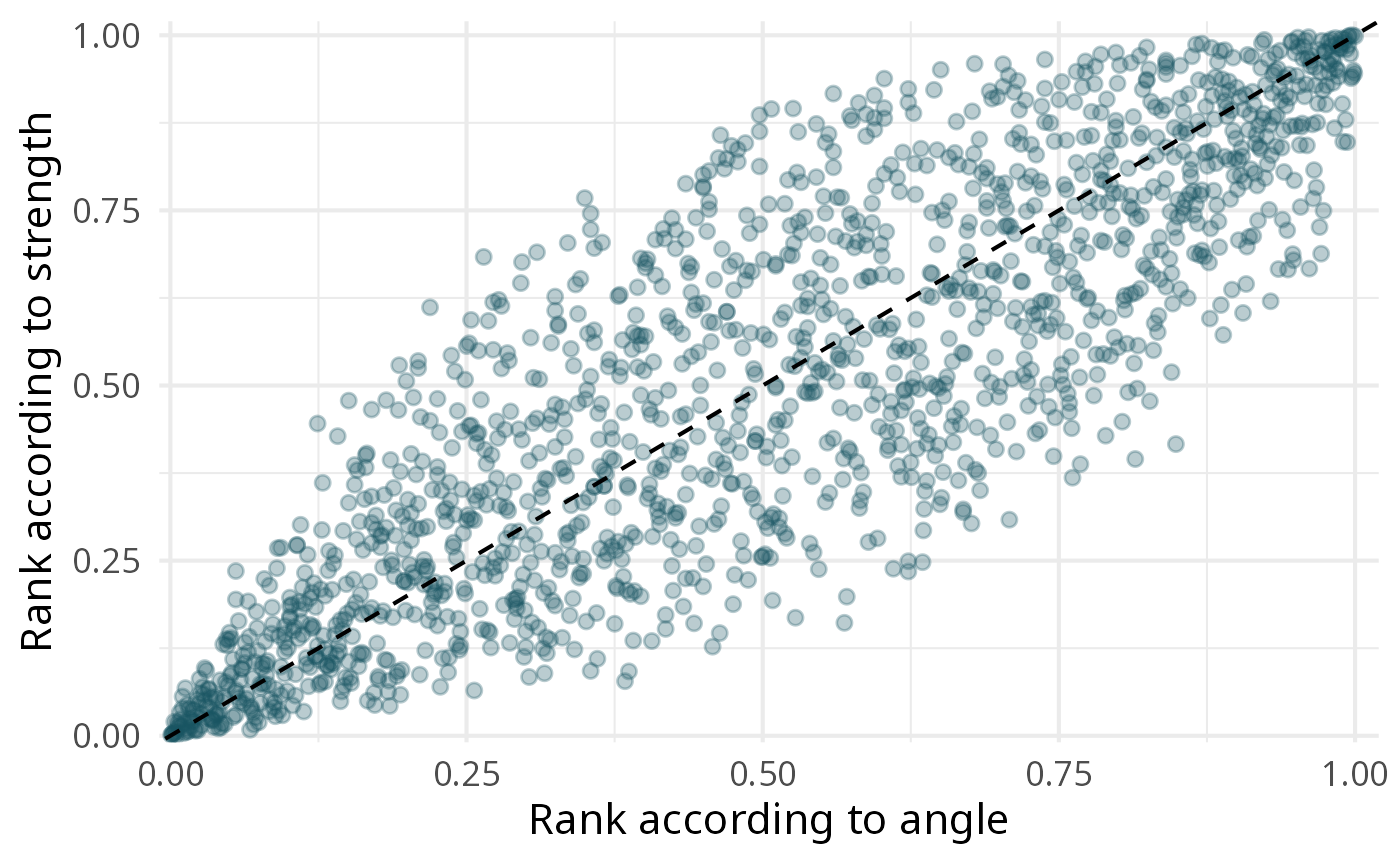
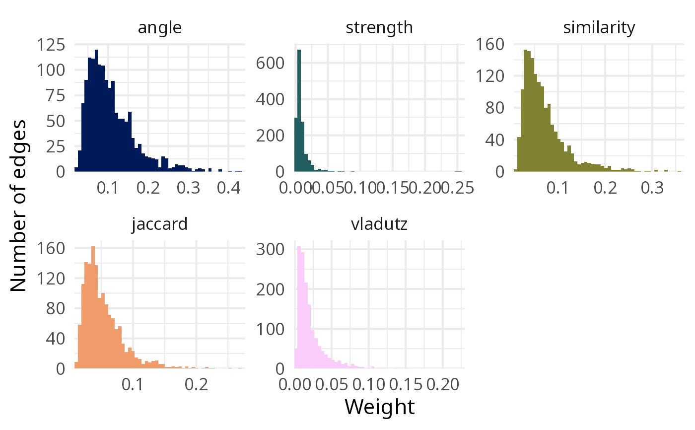
type = "distribution": one histogram of the weights per measure, each with its own horizontal scale (the measures do not share a scale);
type = "scatter": the ranks of the pairs of nodes according to two measures (x and y). Points on the diagonal are ranked identically by both measures; ranks, rather than raw weights, are used because the scales differ.

It needs the ggplot2 and scico packages.

Usage

plot_weights(
  edges,
  type = c("distribution", "scatter"),
  x = NULL,
  y = NULL,
  bins = 50
)

Arguments

edges: A named list of edge tables, for instance from compute_couplings().
type: "distribution" (default) or "scatter".
x, y: For type = "scatter", the names of the two measures in edges (by default the first two).
bins: Number of bins of the histograms.

Value

A ggplot object.

Details

References

Shen S, Zhu D, Rousseau R, Su X, Wang D (2019). “A Refined Method for Computing Bibliographic Coupling Strengths.” Journal of Informetrics, 13(2), 605–615. https://linkinghub.elsevier.com/retrieve/pii/S1751157716300244.

See also

Other tools to compare coupling measures: compute_couplings(), correlate_weights(), merge_weights(), overlap_top_weights(), summarise_weights()

Examples

library(biblionetwork)
edges <- compute_couplings(Ref_stagflation, "Citing_ItemID_Ref", "ItemID_Ref",
                           weight_threshold = 2)
plot_weights(edges)

plot_weights(edges, type = "scatter", x = "angle", y = "strength")